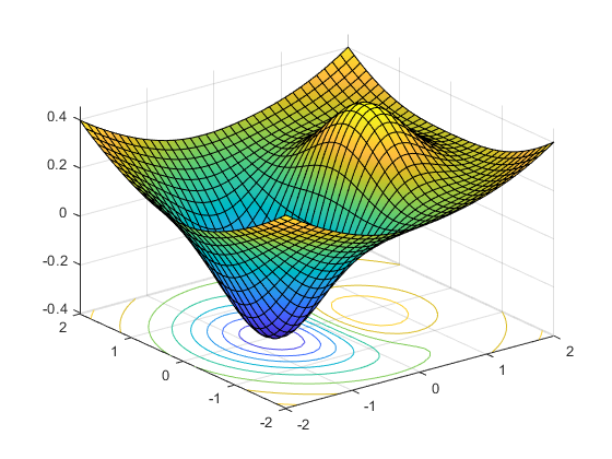
A Bottom-Up Take on Reinforcement Learning up to DDPG
Published:
This is a blog post credit to Tim Krasnoperov and George Stathopoulos
A Bottom-Up Take on Reinforcement Learning up to DDPG
Reinforcement Learning is a popular topic in machine learning that is often hard to understand. A lot of this comes from canonical explanations that follow a “top-down” approach. People are presented the complete package - an abstract environment, action space, rewards, and a mysterious model “policy”, and left to deduce how all this came about. Furthermore, this approach blurs the line between the “learning” and the “reinforcement” of RL. RL at its core is a means of approximating optimal control, an orthogonal concept to neural networks or linear regression. Let’s walk through some problems in optimal control and the closely related concept of dynamic programming. As the complexity of these problems increases, we will naturally and effortlessly stumble upon major ideas in RL: policy gradient, DQN, and the exploration/exploitation tradeoff.
Optimal Control
So, forgetting about reinforcement learning for a minute, let’s consider the problem of playing Tic-Tac-Toe. The board has an initial state which players take turns modifying in hopes of winning the game. An omnipotent player would, for every state, know the best course of action to take to maximize their chance of beating some specific opponent. But what does this mean? This means the omnipotent player has complete knowledge of the entire game tree, and chooses the best strategy for any move the opponent makes. There is nothing to be improved on with this knowledge. It is a solved game. This player has found the optimal control “policy”.
For nine rounds of Tic-Tac-Toe, with $9$ possible actions in the first round, $8$ in the next, and so forth, our game tree can have $9!=362880$ game trajectories. This does not prune games that terminate early, or symmetric game states, but even still it is totally doable on modern computers. The best action to take at a state $s$ and timestep $t$ answers the question: “If I play optimally for the rest of the game after this action, which action should I choose now?”. This should start ringing a bell. This is what the usual $Q$ function in RL tries to describe. Luckily for the case of Tic-Tac-Toe, we can just evaluate all possible strategies from that state, and arrive at an exact solution. But consider the game of chess. Although the number of game states or game trajectories is unknown, Claude Shannon once estimated a lower bound of $10^{120}$. We can no longer traverse the sub-trees. What do we do?
Exact Dynamic Programming and Pruning
The first place to look is dynamic programming. Many “trajectories” of chess games can end up in the same game state. As opposed to re-exploring solved nodes, we simply store them along with their “score”. In the case of chess, this “score” could be the percentage of games won by the optimal policy from that state. This is good, but it will not be enough. The next place to look could be pruning the game tree via symmetries. The following game states of chess are really all the same, so we can treat them as the same state in our DP table.
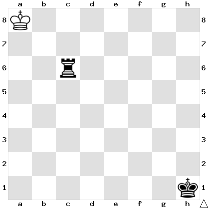
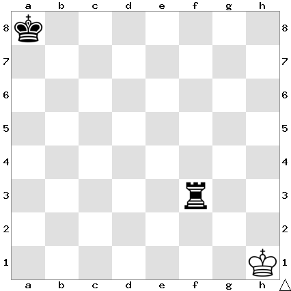
This is also great, but still not even close to enough. What else is there to do? So far, we have only explored exact methods of finding the score at each game state. dynamic programming and symmetric pruning are not approximations. So, where could we bite the bullet and approximate? This is where we really start talking about reinforcement learning.
Approximations and Learning
Monte Carlo Approximations
Perhaps the easiest way to approximate the “expected score” (we can refer to this as the value function from now on) at some state is to do random rollouts from that state. These rollouts can follow from some fixed policy we have, with some form of injected randomness (if the policy is stochastic, then this may not be necessary). This draws out random trajectories in the game tree, which become an unbiased estimate of $J_\theta$ at that state, the value function for the random policy we started with. This is a simple and logical way of approximating what we need, and is used to implement the REINFORCE algorithm.
The REINFORCE algorithm uses these trajectories to compute the gradient of $J$ with respect to $\theta$. We can start with a random policy, and run rollouts at some state $s$. After obtaining the described gradient, we use it to move our $\theta$ value to increase $J$. This clearly alters the policy, as the policy is parameterized by $\theta$. The next time around, we run the rollouts with the new policy, and over time, we perform a stochastic gradient ascent of $J_\theta$ with respect to $\theta$, which ultimately optimizes the policy. This gradient is referred to as the policy gradient.
State Approximations
Consider the following two game states.

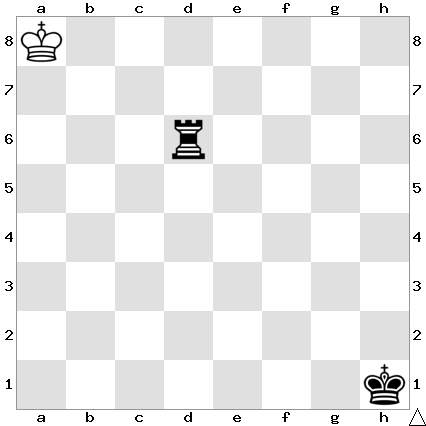
These are most definitely not the same state, but we might expect them to be similar in terms of who this position is advantageous for, and how to act from here. This is where interesting things start to happen. What if we started looking for patterns between these game states and learning them? Could we use similarities between them to draw conclusions about their sub-trees? We could replace (or at least combine) the Monte Carlo simulations with a model that simply learns what are good states and what are bad states over time. Canonically, we are learning the $Q$ function, where the $Q$ function is roughly defined as $Q(s, a) = R(s, a) + J_\theta(s’)$. The $s’$ is the state that would be achieved if we execute action $a$.
Sure, this won’t be exact, but it could be good enough. This would turn the computational cost of evaluating the $Q$ function to the unit cost of running our $Q$-approximation model, and shift the focus towards making an accurate $Q$ function. The obvious idea at this point is to plug in a neural network to model $Q$, and hence we have the idea of a Deep Q-Network, or DQN. Note that by doing so, we lose the nice feature of Monte Carlo simulations which guarantees an unbiased estimate of the gradient we need. As a result, people have found that DQNs can be unstable and never converge.
Deep Q-Networks
DQNs work wonders in a lot of cases. They put all the ideas of symmetry, pruning, and finding patterns into one intelligent function that we learn from data. This data, furthermore, is generated by our simulation, and hence available with rewards in endless quantities.
DQNs segue into another big topic in reinforcement learning. But again, as opposed to explaining it top-down, we will work from the bottom-up. A ubiquitous issue with gradient descent is the fact that it gets trapped in local minima. Neural network gradient descent normally avoids this issue because of the famous result described in “The Loss Surfaces of Multilayer Networks”, where the authors find that local minima are generally close to global minimum for neural networks. This is not necessarily true for the policy gradients we are trying to optimize. In the context of optimal control, our RL algorithm by default finds a greedy solution. Greedy solutions are not always ideal, and as a convenient chess analogy we can bring up the famous queen sacrifice performed by grandmaster Rashid Nezhmetdinov to beat rival Oleg Chernikov in 1962.
One way around this greediness is simply to randomize where we step next. Clearly we don’t want this to be completely random, but rather to strike a balance between “exploiting” a good policy we are developing and “exploring” other options. An easy implementation is to sample from some normal distribution centered on the output of our DQN-outputted action for the state. The variance of this distribution can parameterize how much we value exploitation vs exploration. A small variance means we are usually sampling the “best” action or right around it, and a large variance gives a higher probability of exploring different next actions.
More generally, the DQN begins to take the back seat of controlling the actions, and instead just responsible for quantifying this $Q$ function. This in turns opens up the idea of separating the agent into two parts with a technique called Actor-Critic design. These designs allow for a separation of logic between the “critic” party which is responsible for either the value function or the $Q$ function, and the “actor” party responsible for the policy.
Continuous Control with Deep Reinforcement Learning (DDPG)
Given the practical success of DQN approaches in discrete action spaces, we would like to generalize the idea of using deep learning to solve similar problems with high-dimensional observational spaces but in continuous action spaces. The challenge of directly applying DQN to a problem with a continuous action space is that the $Q$-learning component relies on finding an action which will maximize the value for a given action taken.
Maximizing a continuous action-value function $Q$ requires a somewhat expensive optimization process depending on the action space. For example, an obvious approach is simply to discretize the continuous domain. However, this suffers from the curse of dimensionality: as the dimension of the continuous domain increases linearly, the size of the discretization increases exponentially. Furthermore, a rough discretization can significantly impact the ability to learn tasks involving fine control such as in robotics. Otherwise, in the continuous case an iterative optimization procedure is required at each step of the action-value’s evaluation.
The alternative presented in the paper is what they call a “model-free, off-policy actor critic algorithm” to generalize the DQN algorithm. In particular, the deep nature of the learned $Q$ function allows this method to work in the continuous, high-dimensional action spaces that we were interested in initially. At a high level, the idea is to combine the Deterministic Policy Gradient (DPG) algorithm with DQN. Combining these two techniques involves placing a restriction to the policies that an Actor-Critic algorithm is allowed to use and gives a deep parametrization of the $Q$ function used in the learning algorithm. Since the DQN network is deep, the method is titled Deep DPG, or DDPG for short.
The idea behind DPG is that instead of modelling the policy as a probability distribution over actions, it is instead modelled as a deterministic function of states to actions. Though this might seem initially strange, we can actually view such a deterministic policy as a simple restriction of stochastic policies to delta functions—probability distributions that put all of their weight on a single element of the space. In fact, if the parametrization of the policy is a multivariate normal, this corresponds exactly to the case where every standard deviation associated with the policy is 0 [4]. However, the initial environment state may still be random.
The innovation in the paper is the newfound ability to stabilize the training of the $Q$ function, which was deemed too difficult and unstable for previous $Q$-learning approaches to work in the continuous environment. In particular, as in DQN the author’s of DDPG take advantage of replay buffer sample correlation minimization, temporal difference backups, and batch normalization.
There are two important implementation details. One is that a direct implementation of the Q learning framework is often too unstable when neural networks are directly applied. The actor network, $Q_\theta(s, a)$, and the critic method, $\mu_{\theta}(s)$, are only updated in a soft manner. A hyperparameter $\tau \in [0,1)$ is chosen such that any updates to the hyper parameters is done via $\theta = \tau \theta’ + (1- \tau)\theta$, where $\theta’$ is the update. The other detail that sometimes the deterministic policy does not sufficiently explore the action space. This can be achieved by adding an independent noise process to the deterministic actor policy $\mu(s_t) = \mu’(s_t) + N_t$, where $N$ is drawn from a stochastic process and $\mu’(s_t)$ is the original fully deterministic actor policy. The process may be treated separately to balance between exploration and exploitation. The paper recommends an Ornstein-Uhlenbeck process.
This approach is highly significant (3000+ citations). This significance comes from its relative simplicity and hence robustness of the algorithm compared to other RL methods. It has seen growing applications in portfolio selection, a field that’s intrinsically quite interesting [1, 2].
Conclusion
Going beyond DDPG, there exist extensions to multiple agents using an algorithm known as MADDPG. This could be useful in automatically learning solutions to pseudo-telepathy games. In these cooperative games, there exist multiple separated agents interacting with a referee. The referee then asks them questions which would be impossible to answer unless they had ‘telepathic powers.’ More specifically, they can achieve a level of coordination better than in the nash equilibrium of the (cooperative) game [7]. A famous instantiation of such a game is the CHSH game, where two players guess the xor of two secret bit given to each of them without communicating. Surprisingly, using quantum entanglement between the players there exists a strategy that allows one to win at this game with greater than 85% probability assuming that both input bits are random, while any classical strategy has at most a 75% success rate.
Such games may be formulated as a Semidefinite Program (SDP) and the optimal strategy may be solved directly. However, this has a similar weakness as the exact dynamic programming formulation talked about before: Oftentimes the formulated SDP is exponential in parameters of interest—for example, the number of rounds that are played. Thus, the application of RL in such an instance might introduce novel ways of utilizing quantum mechanics in such games. Quantum mechanics is notoriously difficult for humans to intuitively understand; perhaps an RL approach can be useful.
In sum, RL does not have clear-cut and consistent solutions. There are many approaches for every part in the pipeline, many configurations depending on the environment/action space, and many different sub-algorithms. Sometimes, nothing works. At the end of the day, RL is left with the impossible task of solving problems in PSPACE, and pseudo-greedy approximations may not be good enough.
References:
[1] https://www.semanticscholar.org/paper/A-Deep-Reinforcement-Learning-Approach-to-Fontoura-Haddad/deff7515b984bb7ffe49debb08978f5318a71172
[2] https://rc.library.uta.edu/uta-ir/bitstream/handle/10106/28108/KANWAR-THESIS-2019.pdf?sequence=1&isAllowed=y
[3] https://arxiv.org/pdf/1509.02971.pdf
[4] https://hal.inria.fr/file/index/docid/938992/filename/dpg-icml2014.pdf
[5] http://web.mit.edu/dimitrib/www/RLbook.html
[6] https://lilianweng.github.io/lil-log/2018/04/08/policy-gradient-algorithms.html
[7] https://en.wikipedia.org/wiki/Quantum_pseudo-telepathy
