SATzilla
Published:
This is a blog post credit to Luis Costa, Ajay Natarajan, Kevin Rosa, Eugene Shao, Albert Zhai
Boolean satisfiability
Since the creation of electronic computers, humans have harnessed their blazing computation speeds to solve tremendous numbers of problems. In World War II, the Enigma computer single-handedly gave the Allies an advantage when it started decrypting coded enemy transmissions that humans could not do fast enough. In fact, many problems in the present day and age are quite computationally expensive—i.e. finding the optimal set of items to pack in a suitcase without going over the airline weight limit—and they simply cannot be solved using brute force when the input value gets large (i.e. 100 ton suitcase and items ranging from 1 to 3 pounds) as there are exponentially many possibilities. Many of these problems lie in the NP-complete complexity class.
NP-complete problems are prominent in important real-world applications such as the travelling salesman problem with vehicle routing problems and the vertex cover problem with optimal solar panel placement. Unfortunately, the fastest algorithms that solve NP-complete problems all have exponential asymptotic runtimes, so application of these algorithms to large-scale problems are costly and inefficient.
In computer science, the Boolean satisfiability problem or the SAT problem is the problem of determining whether there exists an assignment of boolean variables that makes a boolean formula true. Similarly, the UNSAT problem is the problem of determining whether the boolean formula outputs false for all assignments of its variables. A boolean formula is called satisfiable if there exists such an assignment and unsatisfiable if not. For example, the trivial boolean formula “(not a) and (a)” is unsatisfiable because no assignment of a can yield true for both a and its negation, so this formula is UNSAT but not in SAT. SAT and UNSAT, which is equivalent to the complement of SAT, are both NP-complete problems by the Cook-Levin Theorem.
SATzilla
There have been many algorithms designed for quickly solving SAT problems, and each variant is best suited for a different type of situation (e.g. number of clauses, number of variables per clause, the distribution of variable appearances across the clauses). However, humans do not know how to choose a solver to deploy in new situations.
In this blog post, we address SATzilla, an algorithm-portfolio-based approach to solving SAT problems. The goal of this methodology is to construct a concise but all-encompassing portfolio of algorithms and learn how to choose which algorithm to use for solving an instance of SAT in the fastest time possible.
The process can be split into an offline and an online component. The offline aspect primarily involves (1) determining useful features for some training set of SAT problems (in early SATzilla versions these included properties of a Variable-Clause graph representing which variables exist in which clauses and a Conflict graph with nodes as clauses and an edge drawn between two nodes if their clauses share a negated literal, just to name a few), (2) portfolio section (selecting a set of algorithms with uncorrelated runtimes on the specific data distribution), and (3) constructing models for each of the algorithm’s predicted runtimes via ridge regression.
The online component involves (1) processing test data and extracting features in the same manner as identified in the offline component and (2) use the offline models to predict which algorithm run times and select the one that runs the fastest for this single test instance.
At a high level, the primary key to this approach is the portfolio-based algorithm approach— because different algorithms may be optimized and more suited towards a certain input type, it may instead be beneficial to determine which of a wide variety of algorithms can run the fastest on the provided input. This instance of the portfolio algorithm approach depends on computed empirical hardness models which estimate the runtime of different algorithms on a given input. This general approach can be applied to other problems in the NP-Complete class outside of SAT, and thus motivates a broader approach to algorithm selection.
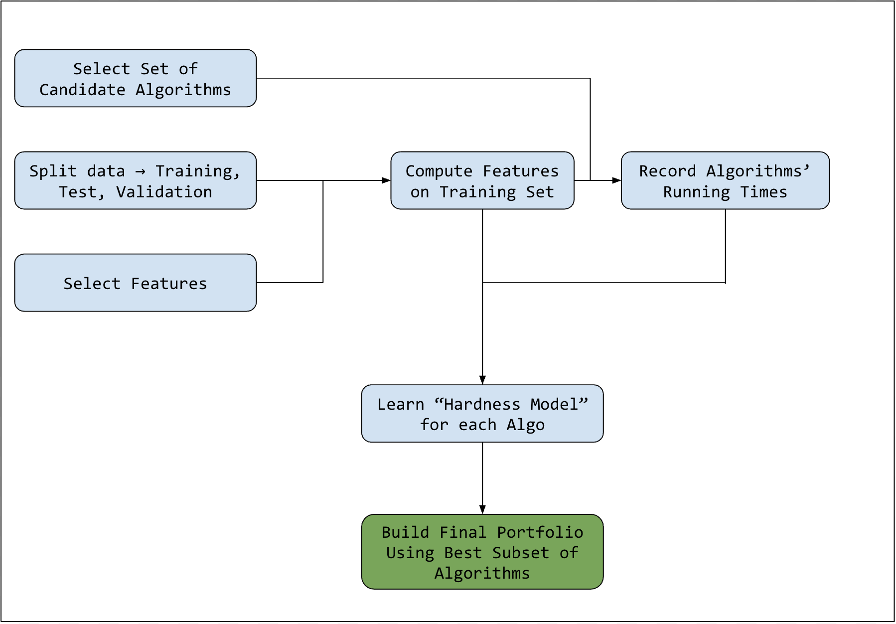 Offline Subroutine Flowchart - Algorithm Portfolio Building
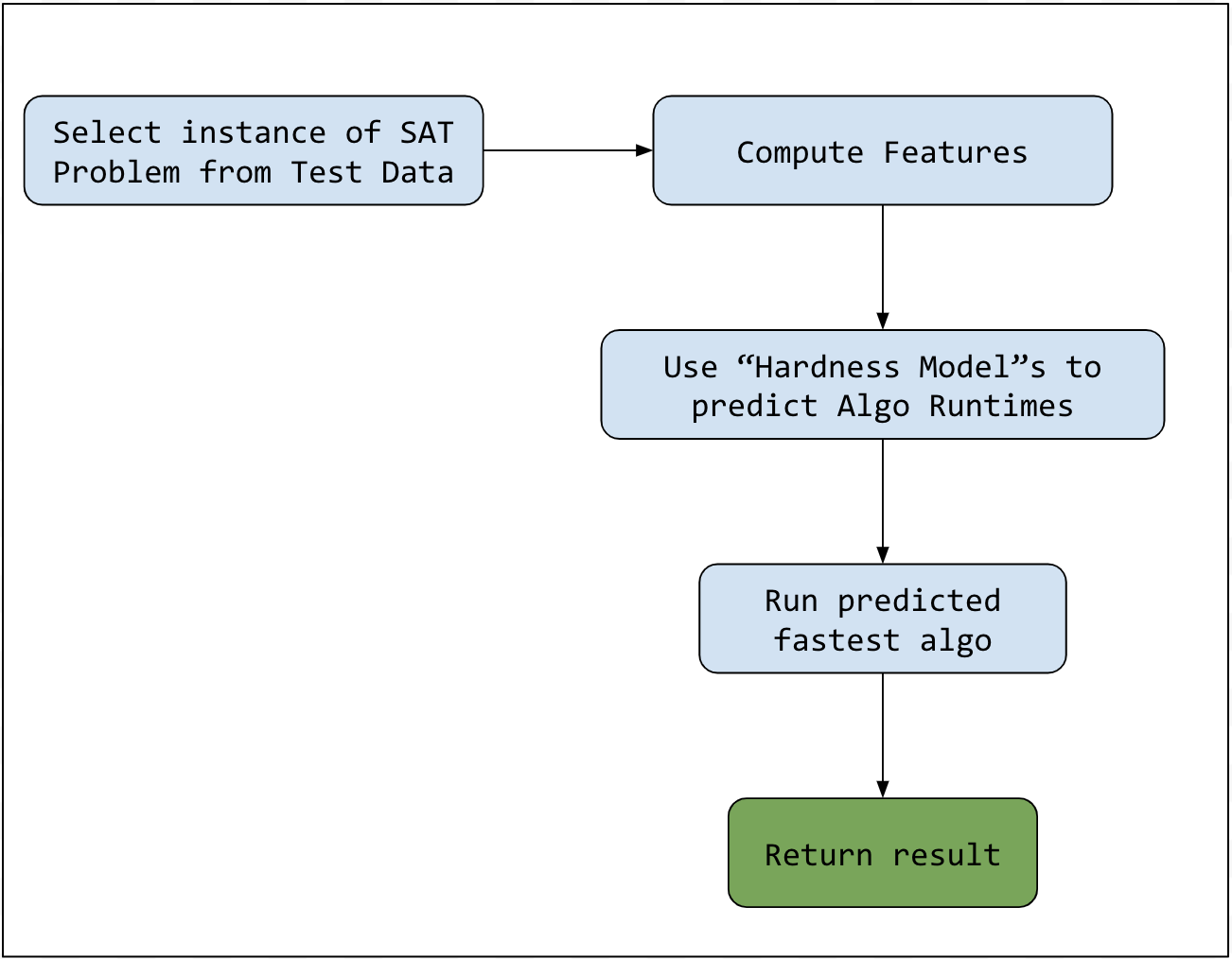 Online subroutine flowchart— SAT Instance Test Algorithm Selection
The above figures are to help visualize the SATzilla process, which is relatively simple. Some common bundles of solvers that are present in many of the versions of SATzilla throughout the years are: OKsolver, Eureka, and Zchaff_Rand, just to name a few. Notably, the Pearson correlation coefficient between OKsolver and Eureka on QCP problems (asking whether given a partially-filled Latin Square, if the remaining entries can be filled in such a manner that would make a valid Latin Square— a problem which is commonly used to evaluate SAT solvers) is low. This low correlation coefficient deems them as good candidates to include in our portfolio.
The main step of developing a SATzilla system is the learning of “hardness models” for each of the candidate solver algorithms. The purpose of these models is to predict the runtimes of the solvers on SAT problem instances drawn from some realistic distribution. To train these models, a dataset of SAT formulae is collected from the desired distribution. Then, a plethora of hand-crafted “SAT features” are computed for each input, ranging from simple properties such as the number of variables and clauses, to detailed results from short runs of search algorithms (see Fig. 3). Ground truth runtimes are acquired by running each candidate solver on each problem input, and then a regression model is fitted to the measured runtimes from the computed features. In the original 2004 version of SATzilla, this was done using simple ridge regression.
To deploy SATzilla on a new SAT formula, all we need to do is to use our models to predict how well each of our candidate solvers will perform, and then run the one which we think will finish the fastest. Now you might have noticed that there is some slight computation overhead induced by the running of all of our hardness models. To combat this, we can use validation right after the training step to select a subset of candidate algorithms for inclusion in our final portfolio. The size of the subset introduces a tradeoff between the selection overhead and diversity of solvers employed.
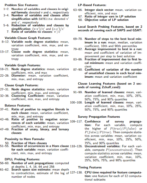 Groups of SAT features. [Source] (http://www.cs.ubc.ca/labs/beta/Projects/SATzilla/Report_SAT_features.pdf)
Winning performance
The SAT Competition is an annual competition for solving Boolean satisfiability problem instances. There are 3 categories of the competition: “industrial”, “hand-crafted”, and “random”, each with their own sets of input formulae. Within each category, there are separate tracks for SAT, UNSAT, and SAT+UNSAT solving. In 2007, SATzilla entered the “hand-crafted” competition, being trained on the problem sets from previous years of the competition. SATzilla won first place in the SAT+UNSAT and UNSAT tracks, plus second place in the SAT track.
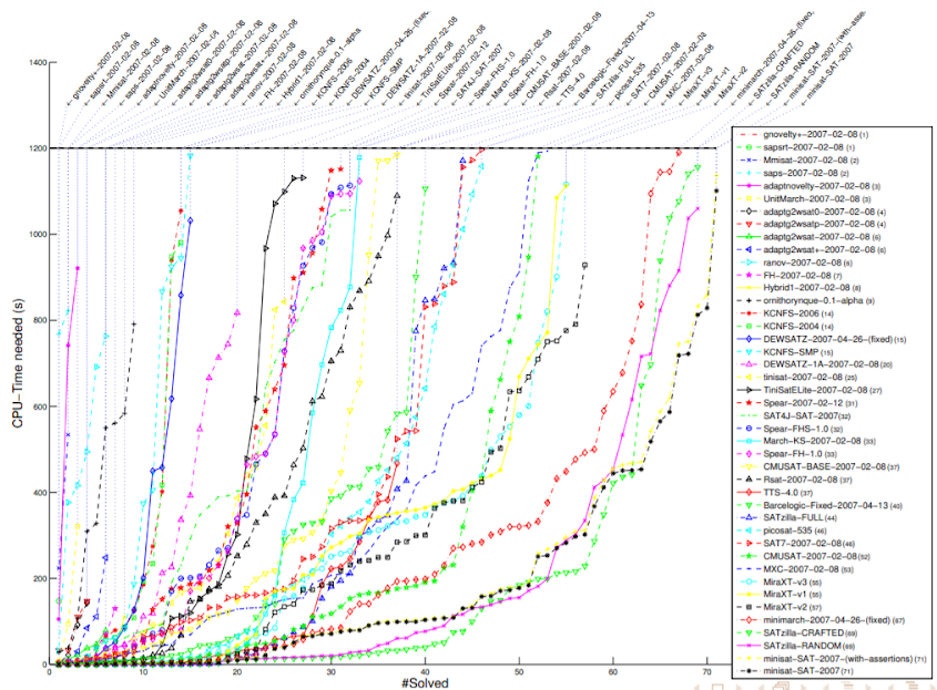 2007 SAT competition (hand-crafted, SAT+UNSAT) results. Lower is better. Source
Theoretical/formulaic derivations
Despite incurring considerable overhead from feature computation and runtime prediction, SATzilla still performs better on average than any of its component solvers. This is due to (1) their uncorrelated runtimes, (2) the relatively large number of them, and (3) the relative accuracy of runtime predictive models. We explore these factors mathematically, describing (A) the general relationship they have to the performance of SATzilla and then (B) how and to what extent each phenomenon is impactful.
A: General relationship between the factors The approximate runtime T of the SATzilla algorithm can be a modeled as follows: $ T = min_{N_f}(r_1,…,r_{N_S}) + t_{compute}N_f + t_{eval}N_S $ where $N_f$ is the number of features used $N_S$ is the number of solvers used $r_1,…,r_N$ are the runtimes of the solvers $min_{N_F}$ is an approximate minimum which is of quality related to the number of features $N_f$ (and their quality) $t_{compute}$ is the amount of time required to compute a single feature $t_{eval}$ is the amount of time required to evaluate a runtime predictive model for a solver
(M2) To minimize 2, we want few features. (M3) To minimize 3, we want few solvers. (M1) To minimize 1, we want many features with low correlation to improve the quality of the minimum and many solvers runtimes with low correlation to decrease the value of the minimum.
The authors of SATzilla address this tradeoff in various ways, including: (M.2) Feature selection based on low Pearson correlation (M.3) Exhaustive solver subset selection based on best performance and low Pearson correlation (T2,T3,M3) Postponing evaluating T.2 and T.3 and using fast, uncorrelated solvers first
B: The factors 1: Uncorrelated runtimes We explore mathematically how low correlation between runtimes minimizes T1. Let $(X_1, X_2)$ be a normal random vector with means $(u_1, u_2)$ variances $(s_1^2, s_2^2)$, correlation coefficient $p$. Let $Y = min(X_1, X_2)$
As appears in source [5], we use that the pdf of $Y$ is $F_Y(y) = f_1(y) + f_2(y)$ where $f_n(y) = 1/\sigma_n \phi((y-\mu_n)/\sigma_n)\Phi(p(x-\mu_n)/(\sqrt{1-p}))$ where $\phi, \Phi$ are the standard normal pdf, cdf. The first moment of $Y$ is $E[Y]$.
If we let $u_1, u_2 = 0, s_1^2, s_2^2 = 1$, we have that $F_Y(x) = 2f_1(x) = 2\phi(x)\Phi(1-\rho/\sqrt{1-\rho^2}x)$ 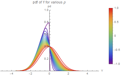
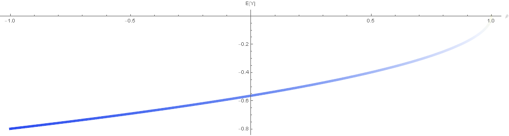
The expected value of $Y$ is $E[Y] = \int_{-\infty}^{\infty}yF_Y(y)dy = \left[(-\sqrt{1-p} Erf(y/\sqrt{1+p}) - \sqrt{2}e^{-y^2/2}Erfc((y-py)/\sqrt{2-2p^2}))/(2\sqrt{\pi})\right]_{-\infty}^{\infty} = \sqrt{(p-1)/\pi}$ 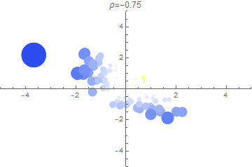
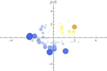
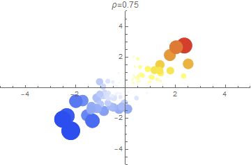
In the 3 plots above, we show a random sample of points $(X_1, X_2)$ for several correlation strengths. A point’s radius indicates the magnitude of the minimum dimension (either $X_1$ or $X_2$) while the color indicates the sign (blue is more negative; red is more positive).
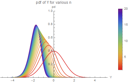
(2) Number of solvers We explore mathematically how the increased number of relatively uncorrelated runtimes minimizes T1. Let $(X_1, …, X_n)$ be a vector of independent (i.e. no correlation) standard normal random variables. Let $Y = min(X_1, …, X_n)$. Since the probability that Y is less than $y$ can be expressed as the probability that not all of the $X_i$ are greater than $y$, the cdf of $Y F_Y$ can be written in terms of the cdf of $X_i F_X$ as $F_Y(y) = 1 - (1 - F_X(y))^n$ In our case then, $F_Y(y) = 1 - (1 - \Phi(y))^n$ In terms of the pdf of $X f_X$, the pdf of $Y f_Y$ at $y$ can be expressed as the probability (density) that any one of the $n X_i = y(nf_X(y))$ times the probability that the minimum of the others is greater than than $y(1-F_{Y[n-1]}(y))$. That is, $f_Y(y) = nf_X(y)(1-F_{Y[n-1]}(y)) = n \phi(y)(1-\Phi(y))^{n-1}$
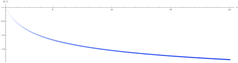
$E[Y]$ can be computed numerically as $\int_{-\infty}^{\infty}yf_Y(y)dy$. Plotting:
(3) Runtime prediction accuracy Finally, we explore mathematically how runtime prediction accuracy minimizes T1.
Let $(X_1, X_2)$ be a vector of independent (i.e. uncorrelated) standard normal variables - 2 runtimes of solvers. Suppose we have predictions $(X_1, X_2)$ called $\hat{X_1}, \hat{X_2}$ made with RMSE of $r$ where the residuals are independent and normally distributed - runtime predictions made by the models (on normalized runtimes). Let $Z = X_1 - X_2$ and $\hat{Z} = \hat{X_1} - \hat{X_2}$ - the true order relation and the predicted one. We now compute the joint probability $P(Z = z, \hat{Z} = z’)$ - revealing how well the runtime predictor preserves the order relation between runtimes (allowing one to choose the lowest one). Since Z is the difference between two i.i.d normal variables, $Z \sim N(0, 2)$ and so $P(Z = z) = \phi(z/\sqrt{2})/\sqrt{2}$
We have then that $\hat{X_1}, \hat{X_2} \sim N(X_1, r^2), N(X_2, r^2)$. Equivalently, $\hat{X_1}, \hat{X_2} = X_1 + \epsilon_1, X_2 + \epsilon_2$ where $\epsilon_1, \epsilon_2 \sim N(0, r^2)$ independently. $\hat{X_1}, \hat{X_2} = X_1 - X_2 + \epsilon_1 - \epsilon_2 = Z + \epsilon_1 - \epsilon_2$ where $\epsilon_{12} = \epsilon_1 - \epsilon_2 \sim N(0, 2r^2)$ Then $P(\hat{Z} = z’|Z = z) = P(Z + \epsilon_{12} = z’|Z=z) = P(z+\epsilon_{12} = z’) = P(\epsilon_{12} = z’ - z) = P(\epsilon_{12}/\sqrt{2r^2} = (z’-z)/\sqrt{2r^2}) = 1/(\sqrt{2}r)\phi((z’-z)/(\sqrt{2}r)) \rightarrow P(Z = z, \hat{Z} = z’) = P(Z = z)P(\hat{Z} = z’|Z = z) = \phi(z/2)/2 \phi((z’-z)/\sqrt{2}r))$ We plot the joint order relation distribution $P(Z = z, \hat{Z} = z’)$ for various RMSE: 


The probability $p_{agree}$ that the estimate gives the correct binary order relation (i.e. greater/less) is the sum of the 2 (symmetrical) ways this can happen: $p_{agree} = P(\hat{Z}>0, Z>0) + P(\hat{Z}<0, Z < 0) = 2P(\hat{Z} > 0, Z > 0) = 2 \int_0^{\infty}\int_0^{\infty}P(Z = z, \hat{Z} = z’)dzdz’ = 2[¼(1 + 2/\pi ArcCot[r])] = ½ + 1/\pi ArcCot[r]$
We plot: 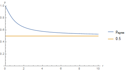
Note that the probability is strictly greater than 0.5, since we assume the predictor is unbiased.
For comparison with the other factors, we are interested in analyzing how RMSE influences the expected minimum runtime Y. We estimate this by assuming that when the order relation is preserved, the runtime chosen is equal to the overall expected minimum of the runtimes (rather than expected minimum given that ). This should produce an overestimate.) That is, $E[Y] \approx p_{agree}E[min(X_1,X_2)] + 1 - p_{agree}E[max(X_1,X_2)]$ From before we know that $E[min(X_1, X_2)] = -\sqrt{(p-1)/\pi} = -\sqrt{1/\pi}$ and $E[max(X_1, X_2)] = \sqrt{1/\pi}$ We plot the estimate.  The red points are $E[Y]$ as estimated by a monte carlo method (i.e. brute force).
Extensions
SAT solvers have a wide range of applications, including problems like formal equivalence checking, model checking, routing of FPGAs, planning and scheduling problems etc. There are even applications in cryptography. Given the wide range and flavor of problems that can characterized as SAT problems, solving instances of these problems in different domains is of great interest. In this section, we give empirical evidence that suggests that there is ample room for advanced ML techniques to improve the efficiency of (both in terms of runtime and level of automation) and extend portfolio solvers like SATzilla.
One of the key parts of the SATzilla approach is the process of engineering features that the model can regress on, to predict algorithm runtimes on a specific problem instance. The authors of the SATzilla papers largely use domain knowledge to identify features that characterize instances of SAT problem. A natural extension to SATzilla would be to try to learn an optimal set of features to use for runtime prediction rather than hand-crafting one. Indeed, Loreggia et al. have a paper focused on completely automating the algorithm selection pipeline using deep learning. Their approach is as follows:
- Convert SAT/CSP problem instances from text files (SAT usually given in conjunctive normal form) to grayscale images. The authors came up with their own procedure for this
- Use these images to train and test a CNN using 10-fold-cross validation. (the trained CNN is a binary classifier).
- For each algorithm in the portfolio, the CNN outputs a value between 0 * (algorithm not at all suited to problem instance) and 1 (algorithm very suited to problem instance). Pick the algorithm with the highest value and run it on the problem instance.
This approach is very interesting and far more automated than portfolio solvers like SATzilla, which rely on hand-crafted features that have been studied and tested for many years. Whilst this CNN approach did not manage to reach the same level of performance as the state-of-the-art portfolio solvers of the time, it did outperform all solvers when just taken by themselves (i.e. no portfolio). This suggests that the CNN managed to extract useful information from the images, which enabled some intelligent mappings from problem instances to solvers.
More evidence of the applicability of deep learning to this area of research comes from [Eggensperger et al.] (https://arxiv.org/pdf/1709.07615v2.pdf) However, they do not tackle the prediction of runtimes of algorithms on given instances - rather, they use deep learning to predict runtime distributions (RTDs) of the features the portfolio solver uses to perform regression. Indeed, one of the extensions the makers of SATzilla made to the original (2007) version in 2009 was to include estimates for the computation time of the features, because during earlier competitions SATzilla would often timeout on feature computation (on over 50% of instances). This extension was just a simple linear regression though. Eggensperger et al. showed that feature RTDs could be well predicted by neural networks. They use a parametric approach, where they consider a certain set of distributions, decide which distribution best models the observed runtimes via MLE and then use a neural network to map features of the problem instance to the parameters of the distribution. Their paper showed that neural networks can be used to jointly learn distribution parameters to predict runtime distributions (RTDs) and obtain better performance than previous approaches such as random forests.
Final thoughts
The success of SATzilla suggests large changes in what the goals of designing new SAT solvers should be. From a practical perspective, the average runtime of individual solvers is no longer important. Rather, the usefulness of a solver may now primarily depend on the uniqueness of the problem instances that it completes quickly. We can see the reason for this by conducting a short thought experiment.
Let’s say that we have two state-of-the-art solvers, A and B, which perform well on different types of problem instances (they have different “easy inputs”). Now imagine that a new solver, called C, is developed. C performs just as well as A, except it also runs as quickly as B on B’s easy inputs. Before SATzilla, this would be a massive achievement, and solver C would quickly find widespread use due to its superior average runtime. However, a well-trained SATzilla will almost certainly perform better. This is because it will know to deploy A on A’s easy inputs and B on B’s easy inputs, and will also solve the easy inputs of its other solvers quickly as well. Furthermore, we won’t gain much in terms of runtime by adding C to SATzilla’s collection, as it is redundant with A and B. Thus, as long as a portfolio like SATzilla remains as the fastest method, the development of solvers like C have little practical value. A weaker solver, with poor average runtime but that runs quickly on some inputs that SATzilla as a whole struggles on, may turn out to be much more useful.
In this sense, we can say that the success of SATzilla, and portfolio methods in general, encourages the research community to take on a “boosting” approach when designing new algorithms. In the boosting paradigm, weak individual models are combined to form an accurate predictive ensemble when the individuals’ areas of effectiveness are sufficiently uncorrelated. Similarly, in SATzilla, slow individual solvers are combined to form a portfolio with low average running time when the individuals’ easy inputs are sufficiently uncorrelated. Just as in boosting, where new individual models should be trained on inputs on which the current aggregate model performs poorly, solver designers may find it most effective to focus on problem instances that the current portfolio as a whole runs slowly on.