Kernel Functions of Gaussian Processes
Published:
This is a blog post credit to Chris Bochenek
Introduction: Qualitative properties of different Gaussian processes
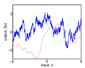
Understanding the kernel function of a Gaussian Process is essential to interpreting its applicability to a give situation, as the kernel function is responsible for restricting the function parameter space for a given model. For example, Figure 1 shows three different functions drawn from three different Gaussian processes. It is evident that these three functions are very qualitatively different. The blue function is very spiky, while the green function is incredibly smooth. The red function is smoother than the blue function, but still has significantly more extrema than the green function.
These differences are not chance coincidence, and the origin of these differences is crucial for interpreting the results of an analysis using Gaussian processes, as choosing a good Gaussian process for a particular application is necessary for good results. If the chosen Gaussian process generates functions that are too spiky, then the analysis will have variance that is too high. On the contrary, if the Gaussian process is too smooth, it may not fully capture the variability of the underlying function. This will lead to an increase in bias. To understand the origins of the differences between these three Gaussian processes, we will refer to Chapter 4 of Rasmussen and Williams, 2006. Figures 1 through 5 are also taken from the text. But first, we will review the basics of Gaussian processes.
# Gaussian processes basics
A Gaussian process is simply a way to state a prior over functions. The only assumption made is that the probability of obtaining function values from a set of points in the domain is jointly Gaussian. In mathematical language, $p(f(\mathbf{x\sb{1}}), … , f(\mathbf{x\sb{N}})) = \mathcal{N}(\mu(\mathbf{x}),\mathbf{\Sigma}(\mathbf{x}, \mathbf{x’}))$. The Gaussian process is specified by two different functions:
1) The mean function – $\mu(\mathbf{x})$
2) The covariance/kernel function – $\mathbf{\Sigma}k(\mathbf{x},\mathbf{x’})$
The mean function, $\mu(\mathbf{x})$, is fairly straightforward to interpret. This represents the expected value of the function. On the other hand, the interpretation of the kernel function is a bit more difficult to interpret. The kernel function, $\mathbf{\Sigma}k(\mathbf{x},\mathbf{x’})$, is the covariance function of the Gaussian process. It specifies based on how correlated $f(\mathbf{x})$ and $f(\mathbf{x’}$ are based off of the values of $\mathbf{x}$ and $\mathbf{x}$. For example, if $f(\mathbf{x})$ and $f(\mathbf{x’}$ are perfectly correlated ($\mathbf{\Sigma}k(\mathbf{x},\mathbf{x’}) = 1$), then $f(\mathbf{x}) = f(\mathbf{x’}$. At the other extreme, if $f(\mathbf{x})$ and $f(\mathbf{x’}$ are not correlated ($\mathbf{\Sigma}k(\mathbf{x},\mathbf{x’}) = 0$), then the values of $f(\mathbf{x})$ and $f(\mathbf{x’})$ have nothing to do with each other ($p(\mathbf{x},\mathbf{x’}) = p(\mathbf{x})p(\mathbf{x’})$).
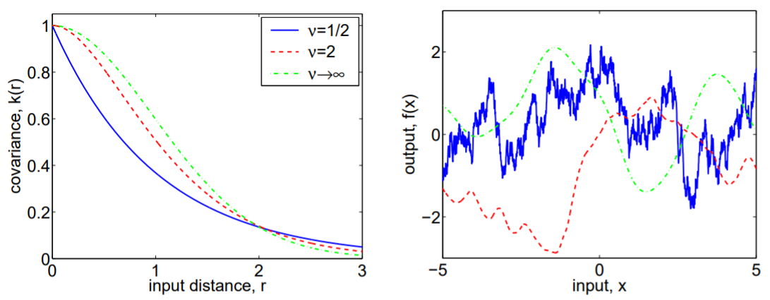
The importance of this kernel function cannot be understated, as it is responsible for the qualitative difference in each of the functions in Figure 1, now shown with the covariance/kernel functions that generated them in Figure 2. We can see that the blue function is highly uncorrelated on small scales, while the green function is highly correlated on small scales, but eventually becomes uncorrelated on large scales. Therefore, the kernel function will define how expressive your Gaussian process is and can essentially be thought of as a bias/variance trade-off. If you are not correlated enough, the spikiness of the resulting functions will increase the variance in your model. If you are too correlated, your model will not capture the full variability of the underlying function, resulting in an increase in bias. In the next section, we will discuss the properties of kernel functions. In the following section, we will go through several different popular kernel functions and explore their strengths and weaknesses.
# Covariance/kernel function properties
Not all functions are a valid kernel. A kernel must be \textbf{positive semi-definite}. Consider a set of inputs $\mathbf{x} \in {\mathbf{x}\sb{1}, … , \mathbf{x}\sb{N}}$. Then the kernel function can be represented by a matrix $\mathbf{\Sigma}$ of size $N \times N$. $\Sigma$ is said to be positive semi-definite if for all $\mathbf{v} \in \mathbb{R^N}$, $\mathbf{v^T\Sigma v} >= 0$. This is equivalent to saying that all the eigenvalues of the matrix are non-negative. This equivalency tells us why kernels must be positive semi-definite. If a kernel is not positive semi-definite, then one of the eigenvalues is negative. However, for a Gaussian process, the kernel represents the covariance matrix of the function, which is assumed to be Gaussian. Since this is a covariance matrix of a multi-dimensional Gaussian, the eigenvalues of the kernel matrix represent the variance along a principle axis of the multi-dimensional Gaussian. However, having a negative variance makes no sense, so all the eigenvalues of the kernel matrix must be positive.
| A kernel is said to be \textbf{stationary} if it is only a function of $\mathbf{x} - \mathbf{x’}$. In other words, the covariance looks the same globally. The variance does not change whether you are at low values of $\mathbf{x}$ or high values of $\mathbf{x}$, only on the relative distance between two points. A kernel is said to be \textbf{isotropic} if it is only a function of $r = | \mathbf{x} - \mathbf{x’} | $. |
| A kernel is a \textbf{dot-product covariance} if $\Sigma (\mathbf{x},\mathbf{x’})$ is a function of only $\mathbf{x} \cdot \mathbf{x’}$. It should be noted that dot-product covariance are not stationary, as they have higher values as $\mathbf{x}$ grows. They are, however, invariant to rotations. This can be seen by the fact that the dot product can be expressed as $ | \mathbf{x} | \mathbf{x’} | \cos{\alpha}$, where $\alpha$ is the angle between $\mathbf{x}$ and $\mathbf{x’}$. If you rotate $\mathbf{x}$ and $\textbf{x’}$ about the origin, the angle between them does not change, so the dot product does not change. |
One way to quantify the “spikiness” of a Gaussian process is through the \textbf{upcrossing rate}. The upcrossing rate is the expected number of times that a Gaussian process with $\mu(\mathbf{x}) = 0$ crosses from below a value $u$ to above $u$. Assuming that the kernel function is twice differentiable, stationary, and continuous, the number of expected upcrossings is $\frac{1}{2\pi}\sqrt{\frac{-\mathbf{\Sigma}’‘(0)}{\mathbf{\Sigma}(0)}}e^{-\frac{u^2}{2\mathbf{\Sigma}(0)}}$.
Two kernels can also be combined to create a new kernel. Some applicable rules are as follows:
The sum of two kernels is a kernel
The product of two kernels is a kernel
The convolution of two kernels is a kernel
The direct sum of two kernels is a kernel
The tensor product of two kernels is a kernel
A kernel function can also be written as a function of its eignenvalues and eigenfunctions:
$ k(\mathbf{x},\mathbf{x’}) = \sum^{\infty}\sb{i=1} \lambda_i \phi\sb{i}(\mathbf{x}) \phi\sb{i}^*(\mathbf{x’}) $
where $\phi\sb{i}$ are the normalized eigenfunctions and $\lambda\sb{i}$ are the eigenvalues. This is simply a diagonalization of an infinite Hermitian matrix representing the kernel function.
A kernel function is said to be \textbf{degenerate} when it has only finitely many non-zero eigenvalues. Thus, it can be written as the sum of finitely many eigenfunctions.
# Covariance/kernel function examples
Squared Exponential Kernel
| This kernel has the functional form $\mathbf{\Sigma}\sb{SE}(r) = e^{\frac{-r^2}{2l^2}}$, where $r = | \mathbf{x} - \mathbf{x’} | $, and $l$ is the characteristic length scale. Since this kernel depends only on $r$, it is an isotropic kernel. An example of a squared exponential kernel is the green kernel in Figure 2. |
One interesting property of this kernel is that the mean functions, $\mu(\mathbf{x})$ are the sum of uncountably many gaussian basis functions with standard deviation $l/\sqrt{2}$, with each Gaussian centered at $\mathbf{x}$.
This kernel function is one of the most popular kernel functions. However, some argue that its smoothness is too strong of an assumption to place on real processes, and thus bias may be increased by choosing this kernel if the real application is not smooth. This problem is addressed in our next class of covariance functions.
Matern Kernels
The functional form of this kernel is as follows: $\mathbf{\Sigma}\sb{Matern}(r) = \frac{2^{1-\nu}}{\Gamma(\nu)}(\frac{\sqrt{2\nu}r}{l})^\nu K\sb{\nu}(\frac{\sqrt{2\nu}r}{l})$, where $l > 0$ is a characteristic length scale and $\nu > 0$ is a hyperparameter that defines how smooth the kernel is, and $K\sb{\nu}$ is a modified Bessel function. This is also an isotropic covariance function.
The covariance functions in Figure 2 are actually from this class. The difference between the kernels is that $\nu = 1/2$, $\nu = 2$, and $\nu=\infty$. The Squared Exponential kernel is actually equivalent to the Matern kernel with $\nu = \infty$. $\nu$ also determines how many times you can mean-square differentiate the kernel. The Matern kernel is k times mean-square differentiable if and only if $\nu>k$. Now we can understand the origin of the difference between the kernels in Figure 2. The blue kernel is not differentiable, and thus produces spiky functions. However, the green kernel is infinitely differentiable (smooth), and produces a very smooth-looking function. The red kernel is one time differentiable, and thus appears somewhere between the blue and green kernels in the spectrum of spikiness.
It should be noted that for $\nu = n + 1/2$, where $n$ is a natural number, the form of the Matern kernel simplifies to the product of a polynomial function of $\frac{r}{l}$ with $p+1$ terms times an exponential of the form $e^{-\frac{cr}{l}}$, where $c>0$ is a constant. This simplification makes kernels of $\nu=p+1/2$ a popular choice. However, it is often difficult to pick between values of $\nu \ge 7/2$ because the data is often too noisy or there is not enough data. Therefore, this leaves us with a class of only 4 popular kernels: $\nu = 1/2, 3/2, 5/2, \infty$.
Radial Quadratic Kernel Functions
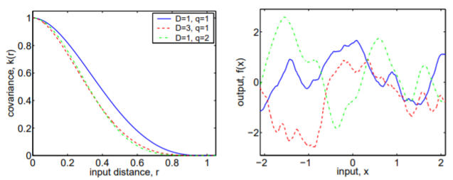
The functional form of this kernel is as follows: $\mathbf{\Sigma}\sb{RQ}(r) = (1+\frac{r^2}{2\alpha l^2})^{-\alpha}$, where $l$ is again a characteristic length and $\alpha$ is a hyperparameter that specifies the distribution of characteristic lengths incorporated into this kernel.
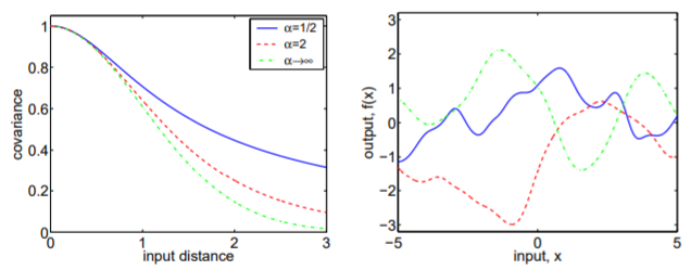
| See, I lied a little bit and said that $l$ was a characteristic length. However, this kernel is formed from taking the sum of squared exponential kernels with different characteristic lengths, where the each characteristic length is weighted by a gamma distribution with shape parameter $\alpha$ and inverse scale parameter $l^{-2}$. Solving the integral $\int \Gamma(\alpha, l^{-2})\mathbf{\Sigma}\sb{SE}(r | l)d(l^{-2})$ yields the functional form of this kernel. You may consider using this kernel when you expect many different correlation length scales to come into play. Figure 3 shows three different radial quadratic kernel functions. |
| You may be inclined to point out that the choice of a gamma distribution seems arbitrary, and you would be absolutely correct. This is just one example of a class of kernel functions which is the sum over squared exponential kernels with different length scales. You can can define any sum of square exponential kernel you want by specifying a probability distribution over $l$: $\mathbf{\Sigma}\sb{SSE}(r) = \int p(l)\mathbf{\Sigma}\sb{SE}(r | l)dl$. |
Piecewise Polynomial Kernels with Compact Support
There is no one functional form for this class of kernels. Having compact support refers to the fact that after a certain distance, the covariance between points drops to zero. This will generate a sparse kernel matrix which has computational advantages. The challenge with these types of functions is proving that they are positive definite. Furthermore, because of their sparseness, they are also not as expressive as other kernels. Figure 4 shows several different functions of the class and Figure 5 shows three examples of this type of kernel and the functions they produce. However, if you are running into computational challenges, it is worth exploring this class of kernel and determining whether the trade-off with expressiveness is worth it.
Dot product kernels
This will be the first class of non-stationary kernels we look at. The simplest dot product kernel is $\Sigma(\mathbf{x},\mathbf{x’}) = \mathbf{x}\cdot \mathbf{x’}$. This is called a homogenous linear kernel. An inhomogenous linear kernal is defined as $\Sigma(\mathbf{x},\mathbf{x’}) = \sigma\sb{0}^2 + \mathbf{x} \cdot \mathbf{x’}$. This form of kernal can be generalized by replacing the dot proudct with a general covariance matrix and raising it to a power: $\Sigma(\mathbf{x},\mathbf{x’}) = (\sigma\sb{0}^2 + \mathbf{x} \Sigma\sb{p} \mathbf{x’})^p$, defining the inhomogenous polynomial kernel. It can be shown that this kernel is degenerate.
| This kernel is typically not chosen for regression problems, as it blows up when $ | \mathbf{x} | > 1$. However, it can be useful for classification problems where the domain is restricted to $[-1,1]$, or problems with binary data. |
String Kernels
| One need not restrict themselves to studying the real numbers. We can also define kernels over other sets, such as strings. Let $\mathcal{A}$ be a finite alphabet, $\mathcal{A^*}$ be the set of strings for this alphabet, and the concatenation of two strings $x$ and $y$ written as $xy$. The length of a string is denoted as $ | x | $. A substring $s$ of $x$ is a string such that $x = usv$ for some strings $s$ and $v$. |
With this in mind, we can define a kernel for strings. Let $\phi\sb{s}(x)$ be the number of times a substring appears in a string, $x$. $\mathbf{\Sigma}(x,x’) = \sum\sb{s \in \mathcal{A^*}} w\sb{s} \phi\sb{s}(x) \phi\sb{s}(x’)$, where $w\sb{s}\ge 0$ is a weight for that particular substring.
| There are a few special cases of this kernel. One, when you set $w_s = 0$ for $ | s | > 1$. This is the bag-of-characters kernel. Two, you can restrict yourself to summing over a subset of $\mathcal{A*}$. For instance, if you only sum over the strings of characters bordered by whitespace, you arrive at the bag-of-words kernel. Three, the $k-$spectrum kernel is when you sum over only substrings of length $k$. |
Conclusion
This concludes our discussion of popular kernel functions and cases where they may be useful. Many other kernel functions have been used, and this is not intended to be an exhaustive list. Furthermore, you may be wondering “How do I pick the optimal hyperparameters and compare different kernels for my application?”. This is a very fair question, and is addressed in Chapter 5 of Rasmussen and Williams, 2006. If you are interested in this topic, I recommend reading that.
