This is a blog post credit to Luka Valencic, Meena Hari, Spiro Stameson, Tarini Singh, and Yasmin Veys

Introduction

The P vs. NP problem is one of the largest open problems in computer science, which asks whether there exists a polynomial time algorithm for problems where the correctness candidate solutions can be verified in polynomial time. While it is widely believed that the class of problems where there exists a polynomial time algorithm, P, is a subset of the class of problems where candidate solutions can be verified in polynomial time, NP, no proof or disproof exists. Within NP, there are is a subset of NP-complete problems, which are a those which can be arrived at from any other NP problem in a polynomial time reduction. As such, NP-complete problems are in NP and are as difficult to solve as any other problem in NP. Many of these problems have practical real world applications, so there is significant interest in creating heuristics that will yield tractable solutions in the absence of an exact polynomial time algorithm. Some examples of NP-complete problems include:

1. The Traveling Salesman Problem: Given a weighted graph, where each vertex represents a city and the edges represent distances between them, find the shortest loop which visits all the cities exactly once. This has direct applications in planning and logistics, as well as other problems like DNA sequence analysis, where distance can be used as a similarity measure.

2. Minimum Vertex Cover: Given a graph, find the smallest set of vertices such that every edge is adjacent to at least one vertex in the set. This has applications in monitoring failures within electronic components.

3. Maximum Cut: Given a connected graph, find the largest set of edges that partitions the vertices into two disjoint subsets. This has applications in statistical physics.

A seminal paper Karp, 1972 on NP-complete problems introduced twenty-one such NP-complete problems, many of which include combinatorial optimization over graphs. While there does not exist a tractable algorithm to solve this class of problems, significant work has been done to engineer algorithms that efficiently compute approximate solutions. Traditional approaches to solving NP-complete problems include exact algorithms, approximation algorithms, and hand-crafted heuristics. There are challenges associated with each approach. Exact algorithms are not effective on large instances of problems, polynomial-time approximations can be slow and inaccurate, and hand-engineered heuristics can be fast and effective, but require a significant amount of specialized knowledge and involve a lengthy process of trial-and-error to construct. As a whole, many previous approaches have not effectively leveraged the fact that in real-world optimization problems, repeated instances of the problem are often solved numerous times. This is particularly true for NP-complete combinatorial graph problems, like the Traveling Salesman Problems.

As such, a recent approach used by Dai, et. al. aims to solve NP-complete problems on graphs by leveraging a combination of reinforcement learning and graph embedding that effectively exploits the recurring structure of real world problems. The learned greedy policy behaves like a meta-algorithm by incrementally constructing a solution, and the action is determined by the output of a graph embedding network that captures the current state of the solution. The graph embedding was created using the structure2vec architecture, and training was accomplished via a Q-learning approach. This novel method resulted in significant improvements in the quality of solutions found through this method compared to standard methods in a diverse range of optimization problems, including Minimum Vertex Cover, Maximum Cut, and Traveling Salesman.

Greedy Algorithms

Greedy algorithms are a class of algorithm which make the locally optimal choice at each iteration in the hopes of arriving at a near optimal solution. A greedy algorithm progresses in a top-down fashion, making one locally optimal choice after another, iteratively building up a solution until it reaches a final solution. The locally optimal choices the greedy algorithm makes is based on a cost or benefit metric, which is most often hand-crafted. As the decision at each step is based on the cost/benefit metric, the quality of the solution arrived at by a greedy algorithm is highly dependent on how well the metric approximates what is the actual best next step.

For instance, for the Traveling Salesman Problem, a simple greedy algorithm would have as its metric the distance from the last city in the current tour to a city which could be added. Using this metric, a tour would be initialized with one city and the city which had the lowest score on the metric would be added to the tour. This would continue until each city was included in the tour. This algorithm does not guarantee that the resultant tour is the shortest one, but hopefully the greedy strategy will achieve a tour close to the optimal one. For some classes of problems, greedy algorithms are guaranteed to yield the optimal solution (i.e. minimum spanning tree). However, greedy algorithms are not guaranteed to yield optimal solutions for every class of problem, though for many problems they can arrive at near optimal solutions, and thus can be quite powerful. Additionally, they have some advantages over other algorithms in that they tend to be simpler and less computationally expensive. This is a major factor in greedy algorithms being a popular choice for solving problems for which finding an optimal solution is not computationally feasible. For instance, a greedy algorithm will run much more quickly than a breadth-first search algorithm which exhaustively explores all possible solutions and thus might be preferable if the solution space is superpolynomial. For graph problems in particular, greedy algorithms are a popular choice to arrive at near optimal solutions quickly.

One NP-hard graph problem that can be approximately solved using a greedy algorithm is the graph coloring problem. The graph coloring problem involves coloring the vertices in a graph with the fewest number of colors such that no two vertices which share an edge are colored the same. The following is the pseudocode which greedily colors a graph whose vertices are labeled $v_1, v_2, \dots, v_N$:

1. Assign the first color to the first vertex $v_1$.

2. For vertices $v_2$ through $v_N$, color it such that the condition is satisfied using the fewest number of colors.

How well the algorithm performs depends on how the vertices are ordered, and there are some heuristics for ordering the vertices such that the greedy algorithm performs better. One example is choosing the next vertex to be the one with the largest number of distinct colors in its neighborhood.

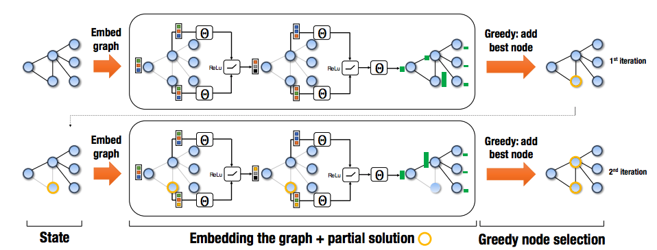
In the approach used by Dai, et. al., a greedy meta-algorithm is used to solve NP-hard graph problems. The greedy algorithm constructs the solution by sequentially adding nodes to a partial solution $S$ until it reaches the full solution. The algorithm chooses the next vertex based on maximizing an evaluation function $Q$. At each step, the algorithm represents the state of the graph and partial solution using the structure2vec graph embedding architecture. In previous research, the evaluation function $Q$ was hand-crafted based on the specific problem, but in this new approach, $Q$ is parameterized and learned.

Graph Embedding Representation

In the context of machine learning, an embedding is a relatively low-dimensional space, where you can can translate high-dimensional vectors to get a more efficient representation as described here. A simple example here generates a word embedding from the one-hot encoding of a vocabulary. The learned embedding is more efficient than the original encoding, since the one-hot encoding is very sparse.

Extending this idea, structure2Vec is a graph embedding network that computes a $p$-dimensional feature embedding $\mu_v$ for each $v \in V$ given the current parital solution $S$, which is an ordered list of vertices. Structure2vec is used to parameterize an estimate of the Q-function, $\hat{Q}(h(S), v; \Theta)$, where $h(S)$ is a helper procedure that maps $S$ to a combinatorical structure satisfying the specific constraints of the problem, $v$ is the candidate vertex to add to the partial solution, and $\Theta$ is a collection of 7 parameter matrices. As an example, a general formulation of structure2vec initializes the embedding $\mu_v^{(0)}$ and updates it recursively according to the following update rule:

where $F$ is a generic nonlinear mapping, $x_v$ is the tag for vertex $v$ that retains features of the vertex, and $N(v)$ is set of neighbors of a vertex $v$ in a graph $G$.

As shown in the above update formula, the embedding space update is carried out according to the graph topology. A new iteration will only start once all vertices in the previous iteration have been updated. The features of $v$ are passed on further through the network and aggregate non-linearly at nodes farther away. After completing the final time step $T$, a node’s embedding will store information about $v$’s $T$-hop neighborhood.

The particular implementation of structure2vec used by Dai, et. al. is given below:

where $\theta_1 \in R^p$, $\theta_2, \theta_3 \in R^{p \times p}$, and $\theta_4 \in R^p$. Observe that ${\theta}_{i=1}^4$ are the learned model parameters for the graph embedding network, and each summation helps aggregate data common among nodes with similar neighbors in $G$. Additional relu layers are included before summing across the neighborhood embeddings in order to increase the efficacy of the nonlinear transforms.

Once the embedding for each vertex has been computed for $T$ iterations, $\hat{Q}(h(S), v;\Theta)$ can be expressed as follows:

where $\theta_5 \in R^{2p}$, $\theta_6, \theta_7 \in R^{p \times p}$, and $[\cdot, \cdot]$ is the concatenation operator. Since $\hat{Q}(h(s),v)$ is computed from the parameters in the graph embedding network, it will depend on every $\theta_i \in \Theta$. The parameters $\Theta$ will be learned, which eliminates the tedious process of hand-engineering the evaluation function and yields a far more flexible approach. Previously, this approach to learning $\Theta$ would require ground truth labels for every input graph $G$, but Dai, et. al. instead trained these parameters with an end-to-end reinforcement learning approach.

Q-Learning

As described here, reinforcement learning works by taking a simulator and exploring sample trajectories for the simulator to estimate high reward actions. In a model-based reinforcement learning approach, the policy mapping states to a probability distribution over actions is known. However, Q-learning differs from this standard approach in that it is model-free, so the policy learned.

Q-Learning operates over a discretized configuration space, with a finite set of actions taken which may be taken at each point in the configuration space. These actions will result in a transition to another state in the configuration space. There is additionally an ‘environment’ which can provides feedback on the quality of the decision made at every step. A policy is learned by repeatedly taking actions at various states according to either the current version of the policy or at random and then updating the policy based on the quality of the next state reached.

In the context of discrete optimization, $Q$-learning is used to form a deterministic greedy policy that selects a vertex $v$ to add to the partial solution $S$, which results in collecting reward $r(S, v)$.

In the work by Dia, et. al., a slight variant of Q-Learning was used. While the Q function is normally updated after looking only one state into the future, in this problem only going one step does not provide a significant amount of information as the graph does not change significantly by just adding one node to the solution which is being built up. As such, the authors would instead look a larger number of steps into the future before updating the Q-function. Additionally, the parameters of the Q-function ($\Theta$ mentioned in the structure2vec embedding) were updated using batch SGD on a randomly selected set of previous iterations instead of normal SGD on the current iteration as this was found to cause the Q-function to converge faster by Riedmiller.

Pseudocode for the Q-learning algorithm used by Dai, et. al. is given below:

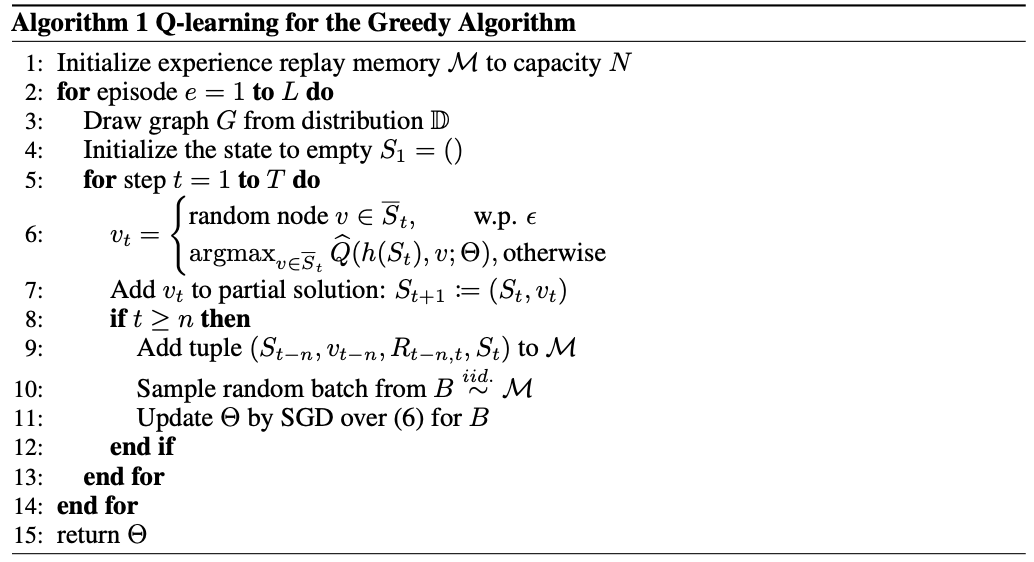
In the above, equation (6) is given by the following:

In standard one-step learning, $y = \gamma \text{max}{v^\prime} \hat{Q}(h(S_t), v^\prime; \Theta))^2 + r(S,v_t)$ for a non-terminal state $S_t$. For multstep learning, as described before, Dai, et. al. use squared loss, but with $y = \sum{i = 0}^{n-1} r(S_{t+i}, v_{t+i}) + \gamma \text{max}_{v^\prime} \hat{Q}(h(S_t), v^\prime; \Theta))^2 + r(S,v_t)$. This approach of using a combination of $n$-step Q-learning and fitted-Q-iteration is more efficient than traditional policy gradient methods, since policy gradient methods require on-policy samples to obtain the new policy after the update.

Results

In Dai, et. al., the authors focused only on learning heuristics for Vertex Cover, Maximum Cut, and Travelling Salesperson problem. The performance of the solver using the learned heuristic (henceforth referred to as S2V-DQN) was compared to a deep learning approach which did not utilize the inherent graphical structure in the graphs (henceforth referred to as PN-AC) as well as some standard algorithms using hand-designed heuristics. The solvers were tested on graphs which have been used to model networks in the real world and for the Traveling Salesperson Problem, on graphs used as part of a challenge to find the best solvers for the Traveling Salesperson Problem.

For both Vertex Cover and Maximum Cut, the S2V-DQN solver was able to find a solution which was not only superior to the solutions of the other solvers, but was also almost exactly equal to the optimal solution. For Vertex cover, S2V-DQN found solutions which were far superior to all the other solvers used while for Maximum Cut, one heuristic based algorithm was very close in performance to S2V-DQN.

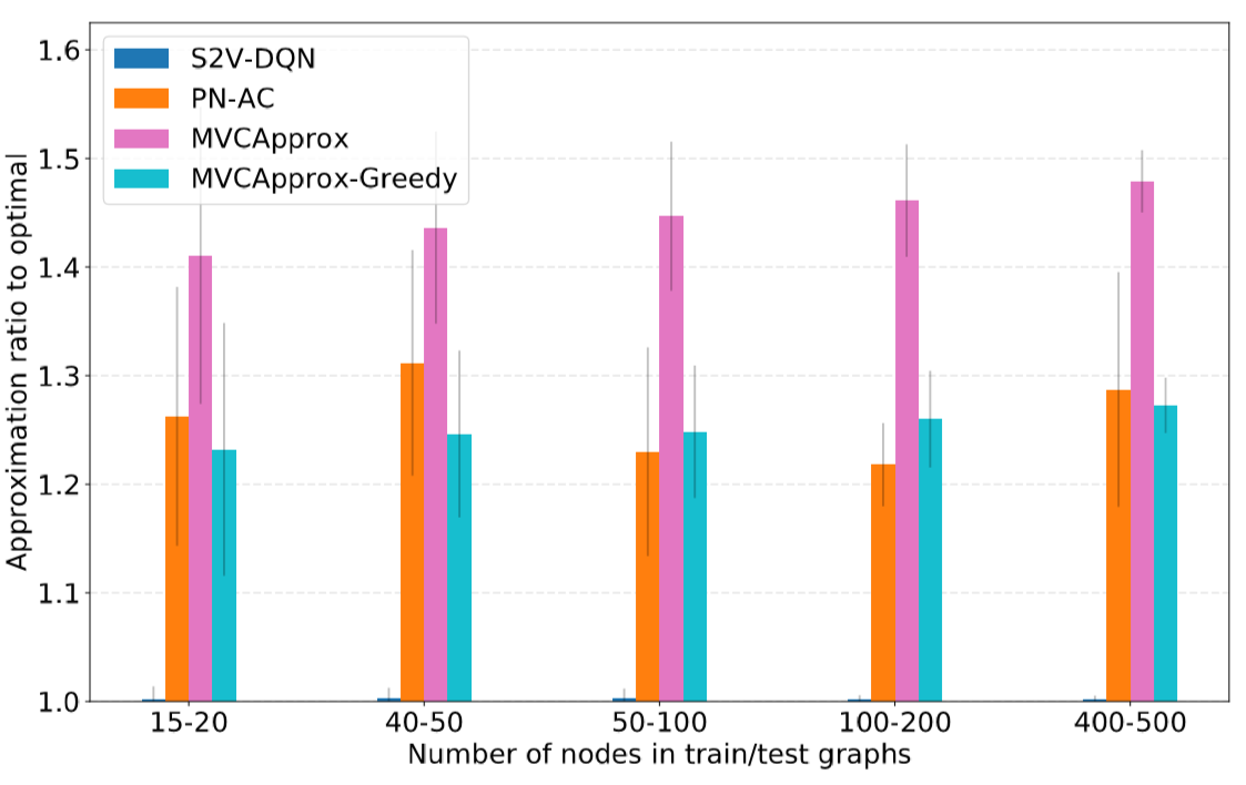
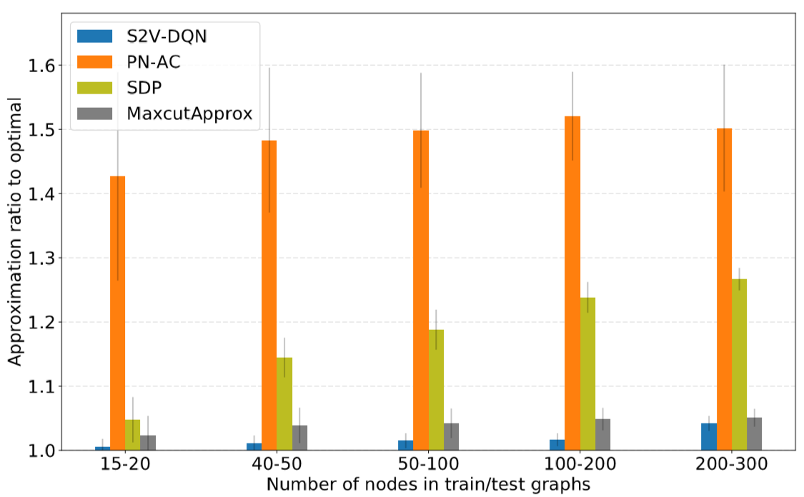
As S2V-DQN was able to find solutions which were very close to optimal, it would seem that the deep learning paradigm was able to learn a very good heuristic for use in the greedy algorithm. The performance of S2V-DQN relative to off-the-shelf solvers suggests that the heuristic for Vertex Cover is significantly better than existing solvers for Vertex Cover and that the deep learning paradigm results in novel insights into the structure of the problem. The similar performance of Maximum Cut relative to a greedy algorithm using a hand crafted statistic suggests that the deep learning did not learn a significantly better heuristic, either because the hand-crafted heuristic is very close to the optimal heuristic or the embedding an neural net was not of a sufficient complexity to uncover a better heuristic.

While S2V-DQN was able to perform better than existing solvers on Vertex Cover and Maximum Cut, for the Traveling Salesperson Problem, the solutions it arrived at were consistently similar to some existing hand-crafted solvers and PN-AC.

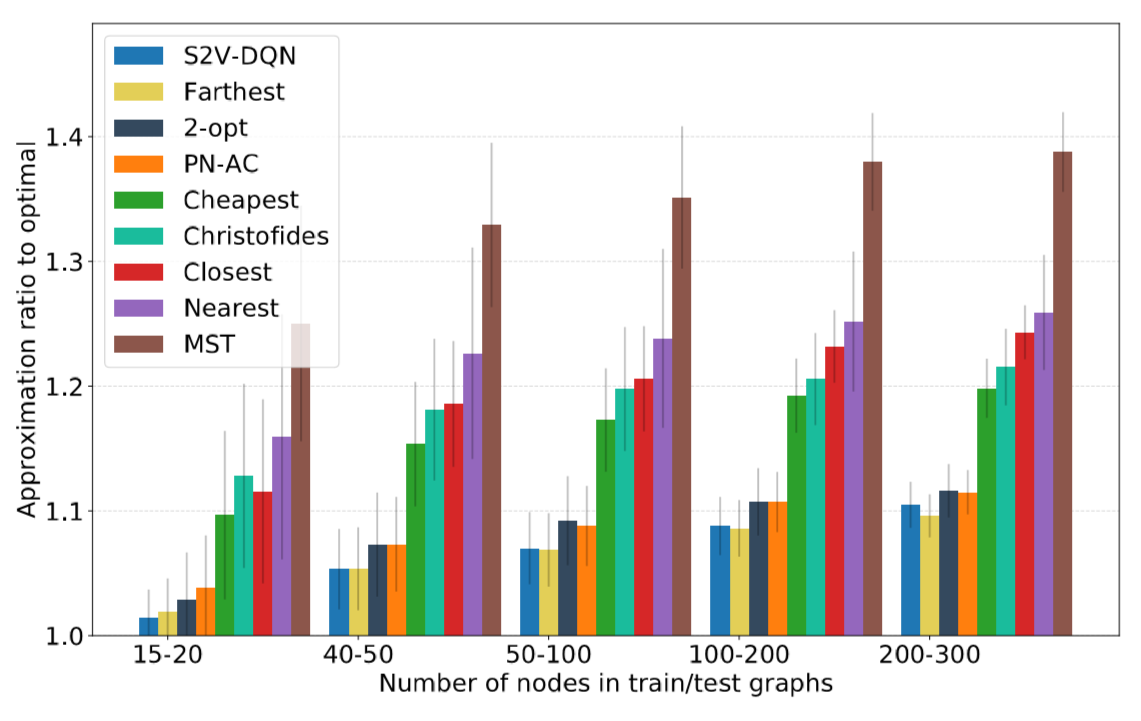
This similarity in the quality of S2V-DQN’s solutions to those of PN-AC suggests that the graphical nature of the Traveling Salesperson problem is not particularly important. This is logical as the graph for the Traveling Salesperson Problem is fully connected and as such the edges only contain distances, which can be fairly accurately modeled in 2D space, which is how PN-AC encodes the information.

While many algorithms which use deep learning are significantly slower than those which do not due to the computational intensity of running input through a neural net, S2V-DQN was able to find a solution faster for both Vertex Cover and Maximum Cut than other solvers which found solutions of similar quantity.

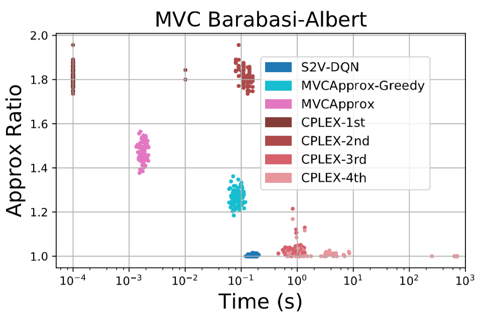
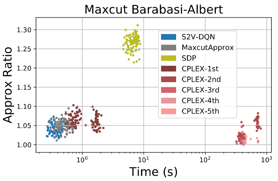
While this fact does come with the caveat that the neural network used to compute the heuristic for S2V-DQN was run on a GPU while the other solvers did not utilize a GPU, this does suggest that S2V-DQN can easily scale to real world applications.

Further Work

While the work by Dai, et al. shows a significant improvement in the field of optimizing combinatorial graph problems, it still has some shortcomings. A few of these shortcomings have already been improved upon in subsequent work.

One drawback with the construction of learned heuristic for a greedy algorithm is that the actual greediness of the algorithm is non-differentiable, which increases the difficulty of learning good solutions. Wilder, et. al attempted to rectify this issue by constructing a fully differentiable reduction from a combinatorial graph problem to a simpler, differentiable problem. As both the reduction and the simpler problem are both differentiable, it significantly eases the difficulty of learning a solution as well as the amount of training examples required.

Another issue with greedily constructing a solution is that even learned heuristics may be unable to make consistently accurate predictions as to what the optimal choice may be when the configuration space is overly complicated. It was possible that this shortcoming appeared in the performance of S2V-DQN on the Traveling salesperson problem as S2V-DQN was outperformed by both the other deep learning model and some hand-crafted heuristics. Chen and Tian attempted to address this issue by modifying an existing solution in local regions based on a choice of update rules. They used learning to both select what region of the solution to update as well as what method to use to update it. This method worked very well on problems with complex solutions spaces, with the problems in the paper being job scheduling, vehicle routing, and expression simplification. This approach had the important advantage over S2V-DQN in that it would reconsider previous decisions it had made at each step, while S2V-DQN did not as it was a greedy algorithm. However, one thing which this paper did not explore was how the initial solution provided to their algorithm affects the speed of convergence and quality of the solution. An interesting possibility would be to explore whether better performance in either category can be achieved by inputting better initial solutions to their solver, possible constructed in a similar manner to S2V-DQN.

Hopefully with further work in optimization of combinatorially hard graph problems, it will become possible to get very close approximations of the best solution, and possibly even high probabilities of obtaining the best solution. This would allow for increases in efficiency in many modern day applications such as delivery truck routing and job scheduling.