Meta-Learning with Gradient Descent

This is a blog post credit to Timothy Yao, Jennifer Yu and Cecelia Zhang

Introduction

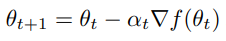
Machine learning tasks can be expressed as optimizing an objective function. Gradient descent serves as a standard approach for minimizing differentiable functions in a sequence of updates following the form:

Vanilla gradient descent is intuitive, but only considers the use of gradients without accounting for second order information. Classical optimization techniques account for this by incorporating curvature information. Current research on optimization involves designing update rules that are optimized for certain subsets of problems. In the realm of deep learning AI, methods are specialized to handle high-dimensional, non-convex problems. Specialization to subclasses of problems is how performance can be improved.

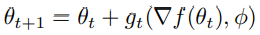
In Learning to Learn by Gradient Descent by Gradient Descent, the idea becomes to replace specific update rules by a learned update rule, called the optimizer g specified by its own parameters φ. The optimizee f becomes of the form:

The update rule g is modeled as a RNN (recurrent neural network) and dynamically updates with each iteration.

The meta-learning idea has been brewing for a while, and recently has been recognized as an important building block in AI. The most general approach involves Schmidhuber’s work where the network and the learning algorithm are trained jointly by gradient descent. More complex cases involve reinforcement learning that trains selection of step sizes and replacing the simple rule with a neural network. Research has explored deeper into the possibilities of neural networks for meta-learning, evolving from NNs with dynamic behavior (without modifying network weights) to now allowing backpropagation of a network to feed into another NN, with both of them trained jointly. The approach in our highlighted paper modifies the network architecture to generalize the approach to larger NN optimization problems.

Gradient Descent

In elementary calculus classes, Euler’s method is commonly presented as a method of approximating values of an ordinary differentiable function by discretely taking successive linear approximations at a certain proportional step away from one another. The process goes like this. Say you have some differentiable function  an initial point  and a terminal point  We can then define the step size to be  for some positive integer  We know what  is, and want to approximate  Using  and  we can find the linear approximation of  With this approximation of  we can then compute the linear approximation of  in a similar fashion. Continuing to do this, we are able to approximate the value of

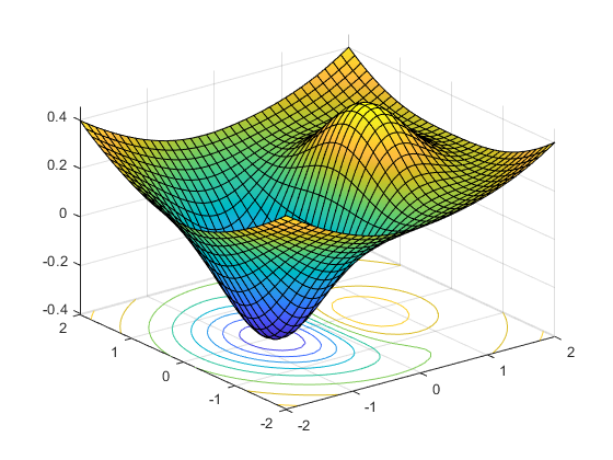
Gradient descent works in a very similar way to the Euler’s method via successive step-wise linear approximations. In the case of gradient descent, we commonly work with multivariate functions with the principle purpose of obtaining the minimum of such functions, i.e. loss functions. Furthermore, with this goal, gradient descent uses the negative gradient of the function at each step, thereby ensuring that the approximations continue to approach the minimum.

The most basic gradient descent might utilize a constant step size. In this case, gradient descent can be thought of as basically Euler’s method applied to multivariate functions and using the negative gradient instead of the gradient. One might notice immediate issues with a constant step size. For example, if the step size is large, then initially, the approximations might approach the minimum quickly, saving computational resources; however, once the approximations hit a critical proximity to the minimum - where more precision might be needed to best approximate the minimum - they might entirely skip over the minimum, oscillating back and forth over the minimum and failing to achieve a better approximate minimum. A step size that is small, on the other hand, might have the exact opposite effect, being able to achieve a better approximate minimum but requiring significantly more computational time to reach it.

Less basic gradient descent might adjust the step size by taking into account second-order information as mentioned earlier. Furthermore, quite advanced gradient descent techniques utilize hand-designed update rules that might not even be strictly convex - making finding a minimum difficult. It follows that we delve deeper into how we might learn such update rules rather than hand-design them in order to achieve optimal optimization.

Fundamental Idea

As mentioned previously, the key goal is to learn an optimization algorithm, or optimizer, for an objective function  that expresses the problem at hand. To do this, the optimizer is modeled as an RNN. Define to be the final optimizee parameters, i.e. the parameters that are input into  to (hopefully) minimize , where  are the optimizer parameters. The optimizer is what updates the optimizee parameters at each time step -  to - so it is natural that the final optimizee parameters  be dependent on how the optimizer has been updating the optimizee parameters  along the way. This is, in turn, determined by the parameters of the optimizer. Understanding this connection, we can rethink the  to be a function of ; necessarily, the final output of  will be determined by how the optimizer has essentially plotted out the course for the optimizee parameters to reach some  It is now that we can formulate the loss function, given a distribution of functions , as a function of the optimizer parameters:

We now take a look at how modeling the optimizer as an RNN allows the dynamic adjustment of how the optimizee parameters are being updated. Define  to be the update rule at time step  i.e. the change between the optimizee parameters at times  and  or explicitly,  where  for some end time  We can then have  be the output of some RNN, which we will denote as  with state  and parameters  We note that the above loss function depends only on the final output of the objective function given the final optimizee parameters  Since the loss function is the primary way we determine how well the optimizer is working, intuitively, such a definition doesn’t provide much information for the optimizer to train on. We thus might want to redefine the loss function to potentially consider how the optimizer performs at each step, i.e.

It follows that

where  can be any nonnegative real number, thought it is common for  for all  Notice that these loss functions equal one another if  for  and  for all other Once again, if this is the case, then the optimizer is only trained on the final step of the optimization, not using any information regarding intermediate steps of the optimization; this implies that the gradients of intermediate steps are zero, making training the optimizer through methods, like Backpropagation Through Time, inefficient.

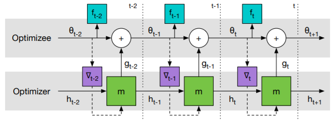
As with many problems, we now want to minimize the loss function, and we do so through gradient descent on  In order to avoid computing second derivatives of  we make the assumption that the gradient of the optimizee  and the optimizer parameters  are independent of one another, implying that  Sampling a random function  from the given distribution, we then compute the gradient estimate  using applying backpropagation to the computational graph below. Notice that by our assumption, we need only compute the solid edge gradients.

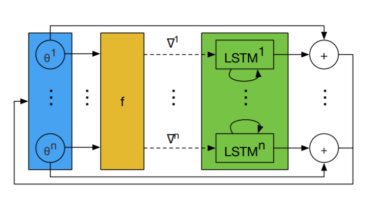
One problem that does arise from using the RNN model is that it requires huge hidden states and an enormous set of parameters, in the case where thousands of parameters are being optimized. In order to circumvent this obstacle, a coordinatewise network architecture is used, where the optimizer separates and operates on the individual coordinates of the parameters. This allows for a smaller network, and the optimizer can now be independent of the order of the parameters in the network. Each coordinate is updated using a two-layer Long Short Term Memory network which relies on previous hidden states and the optimizee gradient for the coordinate. This idea is referred to as the LSTM optimizer, as seen in the figure below, which shows a single step in the LSTM optimizer and how there are separate LSTMs that share parameters and have their own hidden states.

Examples and Experiments

A variety of experiments are performed to test the effectiveness of the learned optimizer in comparison to optimizers that were created by hand. Each LSTM has 20 hidden units per layer and uses ADAM for minimization of the loss function.

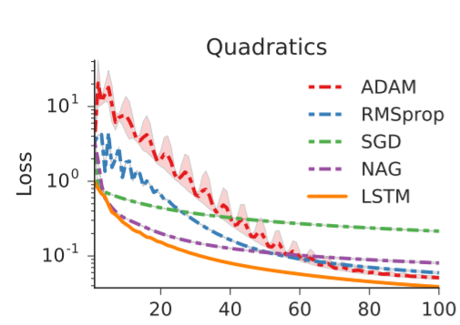
In the first experiment performed, the optimizer is trained on synthetic 10-dimensional quadratic functions of the form

where W is a 10x10 matrix and y is a 10-dimensional vector. Functions are randomly generated for the optimizer to train on for 100 steps and then tested on separately created functions from the same family. The learning curves for several different optimizers are seen below, which shows the average performance over several test functions over an increasing number of steps. Since the LSTM has a steeper downward trend that occurs faster than the trends for the other optimizers, this suggests that use of the LSTM optimizer could be more effective than other standard hand-crafted optimizers.

Another interesting application of this method is its possible use in Neural art, which is when convolutional networks are used to transfer artistic style. The complexity in neural art stems from how each style and image input creates a unique and difficult optimization problem. The problem is defined as

where we have c as the content image and s as the style image, and the minimizer of f is the styled image. The last term works as a regularizer in order to ensure smoothness of the styled image, while the first two terms work for creating content and style that match c and s. The optimizers were trained using only one style image and 1800 64x64 content images from ImageNet, where 100 content images were used for testing and 20 content images were used for validation.

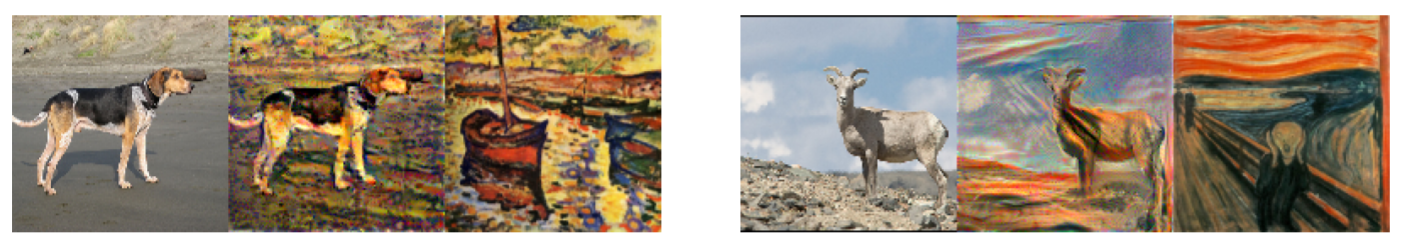
The above images are example inputs and outputs, where the left image in each group is the content image, the right is the style image, and the center image is the one generated by the LSTM optimizer.

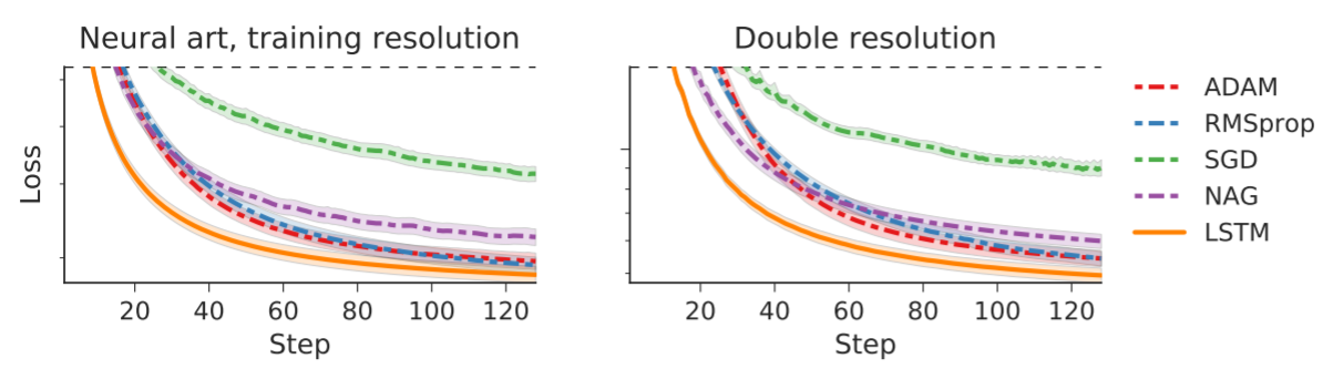
The above figures compare optimization curves for Neural Art using the LSTM optimizer and other handmade optimizers at a log scale. Both graphs have been cropped to the section that is more interesting. The left figure uses testing images that are at the same resolution as the images used in training, while the right figure uses testing images that are double the training image resolution. Since the curve for the LSTM optimizer has a lower loss at all steps, it suggests that this method of optimizing is promising in applications relating to Neural Art.

Follow-up work

With meta-learning continuing to be a prolific field within machine learning, the ideas we have presented from the paper Learning to learn by gradient descent by gradient descent have developed related work, especially with regards to enhancing meta-learning algorithms and designing better neural network architectures. One of the key principles presented by the paper we have delved into was that improvements related to the learned nature of the optimization algorithm were specific to classes of problems at the expense of other classes of problem, i.e. no one learned algorithm could see such improvements to all models it was applied to. The work of Finn, et al. [2017], for example, worked to amend such specificity, attempting to formulate an algorithm that was “model-agnostic,” i.e. could work on any model trained with gradient descent and a variety of learning problems. Furthermore, we have seen improvements to neural network structures as a result of this meta-learning scheme, as demonstrated in the work of Zoph and Le [2017]. Finally, such improvements to neural networks boost the potential for the continual development of artificial intelligence to gain human-like traits, as discussed by Lake, et al. [2016].

Final Thoughts

We have seen through the definition of this new learning problem and the variety of research recently performed that meta-learning is a promising new field that suggests future optimization algorithms can be learned rather than handcrafted. In addition, through the empirical results found by this paper, we find that learned optimizers may perform better than hand-crafted optimizers in certain applications, which could allow enhanced performance of future machine learning models. However, it is important to be cautious in our praise of the experiment results, because of the limited reach of the experiments performed in this paper. Further research is needed in testing a greater variety of model applications.

References

Andrychowicz, M., Denil, M., Gomez, S., Hoffman, M. W., Pfau, D., Schaul, T., … & De Freitas, N. (2016). Learning to learn by gradient descent by gradient descent. In Advances in neural information processing systems (pp. 3981-3989).

Finn, C., Abbeel, P., & Levine, S. (2017, August). Model-agnostic meta-learning for fast adaptation of deep networks. In Proceedings of the 34th International Conference on Machine Learning-Volume 70 (pp. 1126-1135). JMLR. org.

Lake, B., Ullman, T., Tenenbaum, J., & Gershman, S. (2017). Building machines that learn and think like people. Behavioral and Brain Sciences, 40, E253. doi:10.1017/S014 0525X16001837

Zoph, B., & Le, Q. V. (2016). Neural architecture search with reinforcement learning. arXiv preprint arXiv:1611.01578.