Meta-Learning
Published:
This is a blog post credit to James Deacon, Eric Han, Alycia Lee, Emma Qian, Daniel Zhou
Introduction: What is Meta-Learning?
Meta-learning is a subfield of machine learning that tackles the problem of “learning to learn.” Oftentimes, machine learning models (in particular, deep learning) require a huge number of training examples to learn to perform a specific task well. On the other hand, we as humans possess the capability to enhance our own learning efficiently: to learn new skills and solve new problems. For instance, children are able to tell dogs apart from cats after seeing them only several times. This is the essence of meta-learning: to train a model on a variety of learning tasks so that it can learn to solve new tasks quickly and with few training examples. Learning tasks refer to any classic machine learning problem, such as supervised learning, classification, regression, reinforcement learning, etc.
Meta-learning models are expected to be able to generalize well to new learning tasks not seen during training. A simple example of meta-learning includes a classification model trained on images of animals that are not dogs that is asked to identify dogs in test images after only being shown a few images of dogs. From Oriol Vinyal’s talk at NeurIPS 2017, the idea of the training setup for meta-learning, specifically, few-shot classification (which is discussed further in the Discussion and Further Work section), is:
We are given a dataset $D$ with a complete set of labels $T$. The dataset consists of feature vectors and labels, $D=$ \{$(\textbf{x_i}, y_i)$\}. Let $\theta$ denote parameters of the classifier, which outputs a probability of label $y$ being attributed to a feature vector $\textbf{x}$, $P_\theta(y|\textbf{x})$.
- Sample a set of labels $L$ from $T$
- Sample a support set $S$ from $L$, and a training batch $B$ from $L$
- Optimize the batch (use it to compute loss, and update parameters via backpropagation), then go back to step 1.
The optimal parameters are chosen as:
Each pair $(S,B)$ can be considered as a single data point. Therefore, the training routine is constructed so that the model can generalize to other datasets after training.
Recent Work in Meta-Learning
The concept of meta-learning was first described by Donald B. Maudsley in his PhD dissertation (1979) as, “the process by which learners become aware of and increasingly in control of habits of perception, inquiry, learning, and growth that they have internalized.” Later on, John Biggs (1985) defined meta-learning as the state of “being aware of and taking control of one’s own learning” in his publication in the British Journal of Educational Psychology.
Since then, much progress has been made in the development of meta-learning methods–particularly, in the past few years. The deep learning space has witnessed an increase in exploration and research of such techniques. Most methods have centered on three approaches: 1) model-based, 2) metric-based, and 3) optimization-based.
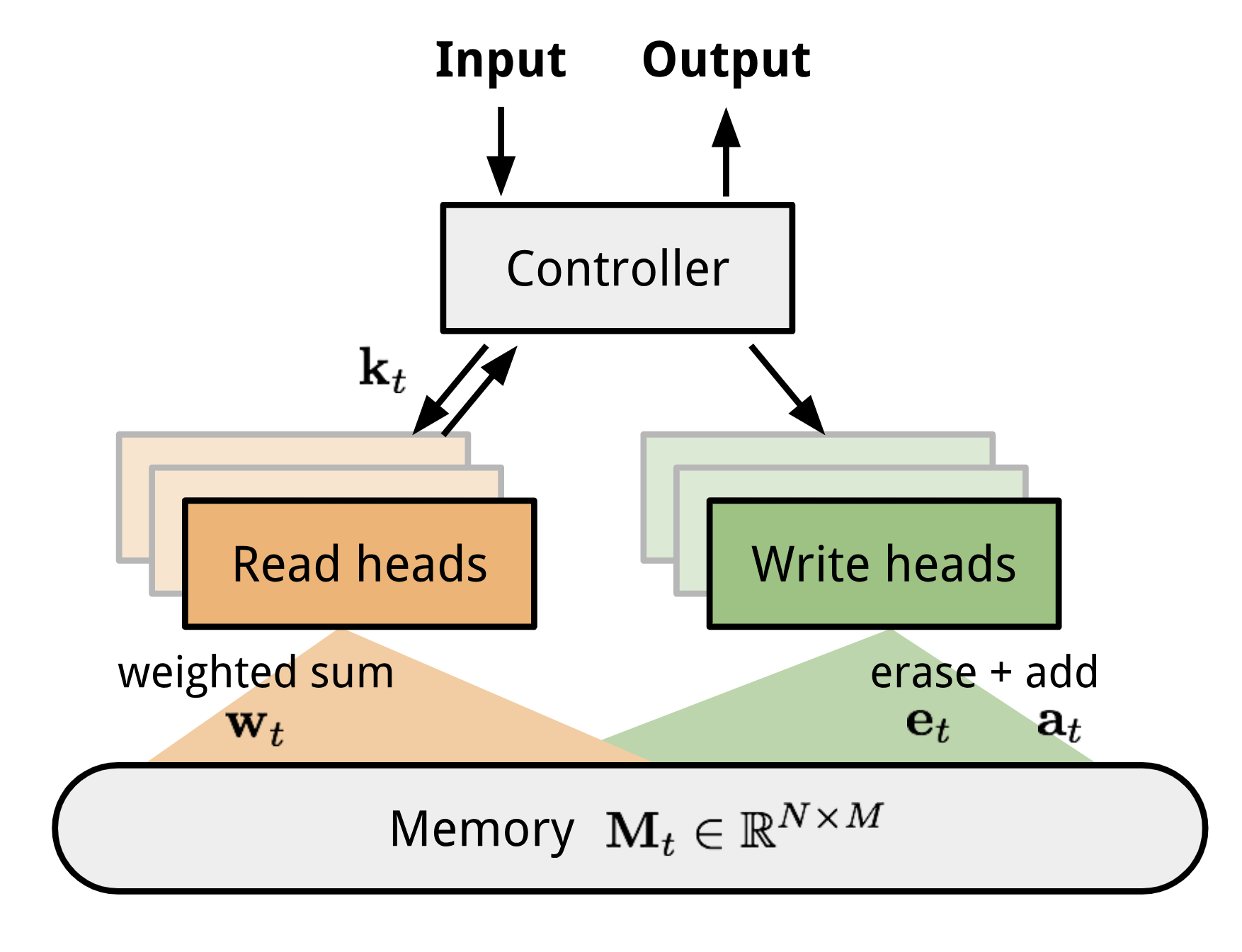
Model-based models perform parameter updates with very few training steps, and do not assume the formulation of $P_\theta(y|\textbf{x})$. An example is a Memory-Augmented Neural Network (MANN), which is capable of encoding new information quickly, and adapting to performing new learning tasks. MANNs comprise a model architecture class that uses external memory to facilitate the learning of neural networks. Neural Turing Machines (NTM) and Memory Networks both belong to the MANN architecture class. To train MANNs for meta-learning, Santoro et al., 2016 proposed a method to present labels at a later time step in order to force memory to contain information longer. This forces MANNs to memorize information from a new dataset until the label is presented, and then reference back to previous information in order to make a prediction. Another model-based meta-learning method is the Meta Network (MetaNet), which is trained for rapid generalization on new learning tasks with few training examples.
Metric-based models are similar to nearest neighbors algorithms, such as kNNs and k-means clustering. The aim is to learn a metric or distance function over objects (i.e. kernel). The kernel function determines the similarity between two examples, and serves as a weight on labels: The formulation of the kernel depends on the task to be performed.
Metric-based models include Siamese neural networks, which consist of two twin networks with identical weights and parameters, joined together by a neuron. During joint training, each network extracts features, and the outputs are evaluated by the joining neuron, which learns how pairs of input examples relate. Convolutional Siamese neural networks have been used for one-shot. Other metric-based models include Matching Networks and Relation Networks, which are similar to Siamese networks.
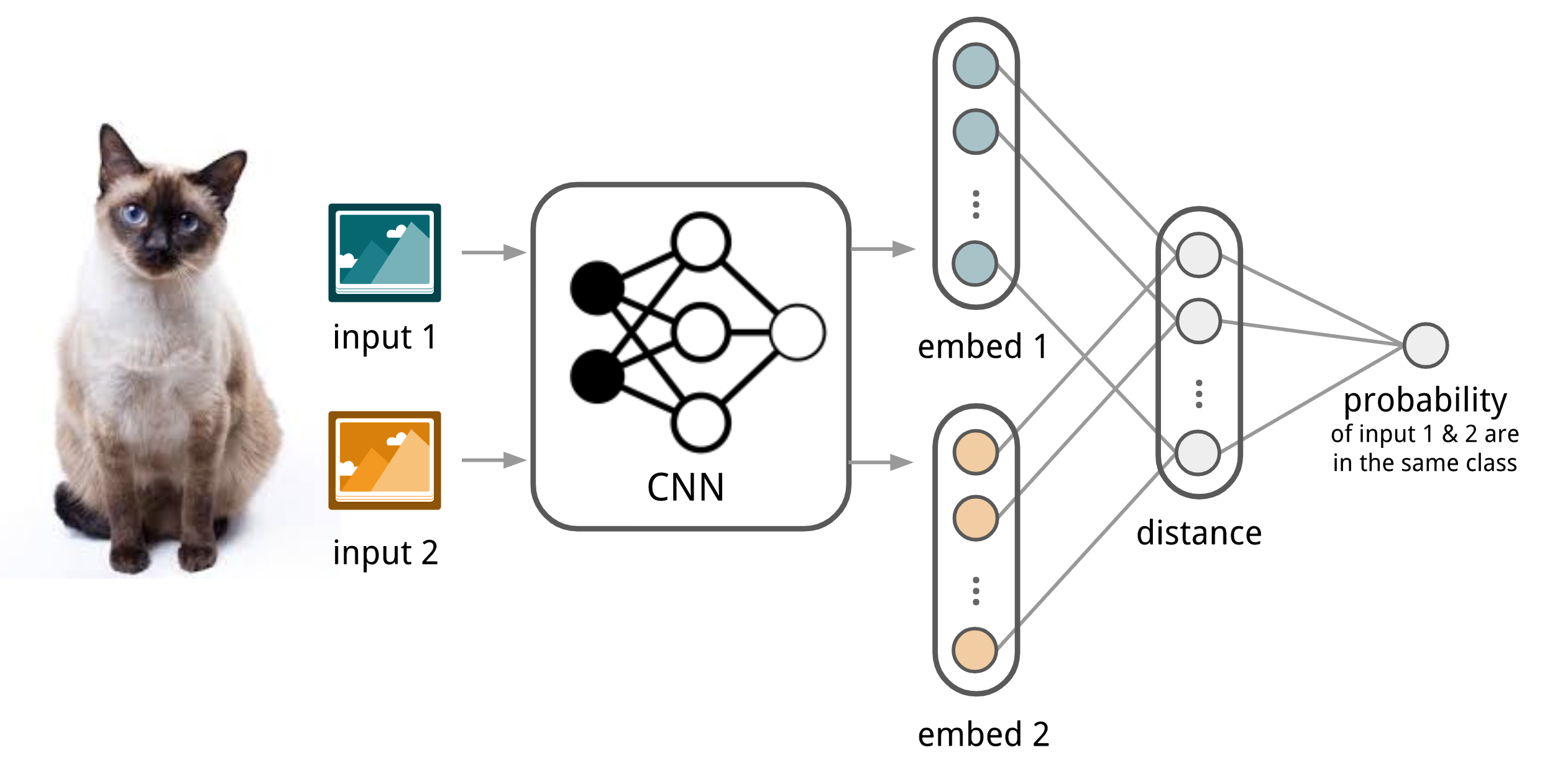
Convolution Siamese neural network architecture used for image classification.
The goal of optimization-based models is to modify the optimization algorithm to ensure that a model can learn well with few training examples. For instance, deep learning models use backpropagation of gradients to optimize and learn, which require many training examples and many time steps to converge. A Long-Short Term Memory (LSTM) “meta-learner” was proposed by [Ravi and Larochelle (2017)] (https://openreview.net/pdf?id=rJY0-Kcll), which learns an exact optimization algorithm used to train another neural network, called the “learner,” in a few-shot learning scheme. The meta-learner was selected to be an LSTM due to similarities between how cell-states are updated in an LSTM and how gradients are updated via backpropagation.
We describe an optimization-based approach, Model-Agnostic Meta-Learning in greater detail.
Recent Advances: Model-Agnostic Meta Learning
Model-Agnostic Meta Learning (MAML) is a recent advancement in meta-learning. It only assumes that the model is trained by a gradient descent procedure, a very general assumption. MAML can be applied to regression, classification, and supervised learning. It provides significant benefits by “pre-training” a model on a variety of tasks so that the model is capable of few-shot learning, i.e. converging quickly on specific problems with little data.
Let’s first define some terms. We begin with the model, which is simply a function that maps observations $x$ to a label $y$: There are learning tasks to which the model is applied, composed of a loss function, a distribution over initial observations (initial state distribution), and a transition distribution on observations between different time steps. Note that a task is an entire problem definition, not an example of data.
The initial state distribution allows us to sample a first data point. We then continuously sample additional points based on the transition distribution, which gives the probability of seeing a data point at the next time step given data from the previous time step. These points will all be correlated. If we want a new independent data point, we go back to the distribution on initial observations and sample from there.
$H$ can be thought of as the number of points that are in a batch. To create a batch, we sample a point from the initial state distribution, then $H-1$ points from the transition distribution. The loss function takes this size $H$ batch and returns a real-numbered loss.
To review, we have a model, which can be applied to a learning task. The probability distribution over learning tasks is encoded in:
We will train the model on all tasks in $P(T)$, accounting for the probability of seeing each task.
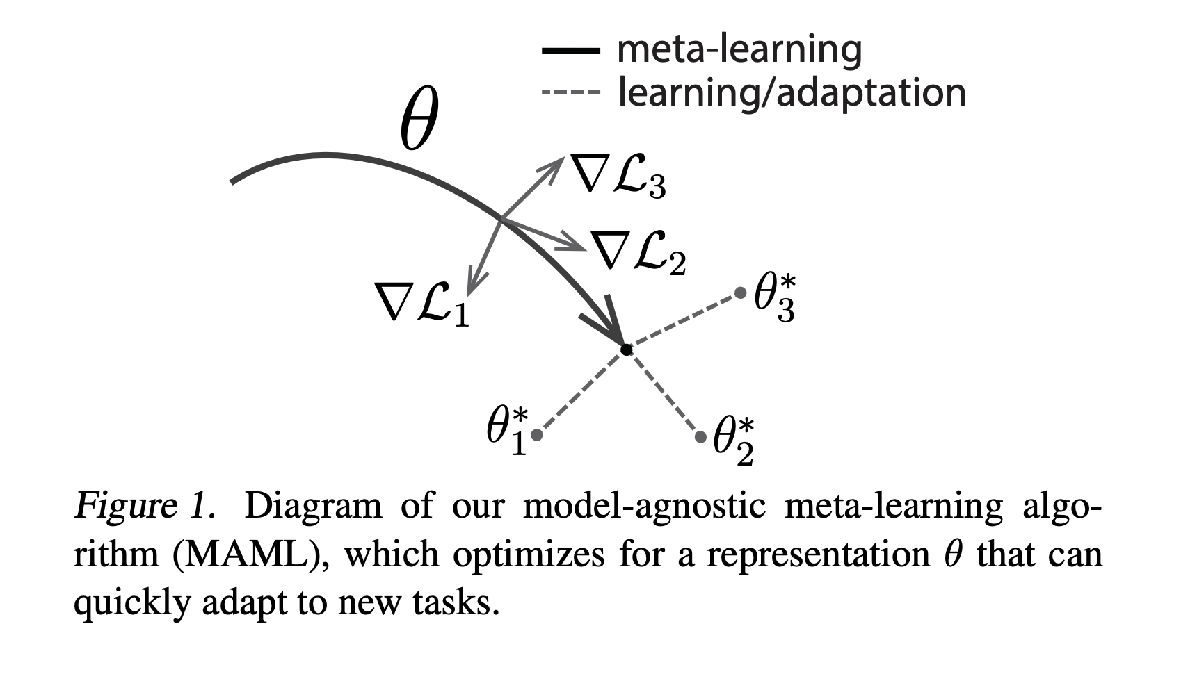
The core idea of MAML is to train the model’s initial parameters so that the loss is most sensitive to gradient updates when the model is trained on a specific task. For example, a neural network could learn general structures that apply to all tasks in P(T). When the network is trained on a specific task, it already has a general understanding of the problem space and quickly learns the specifics of the task. For a clearer definition, let’s look at the objective function of the MAML algorithm.
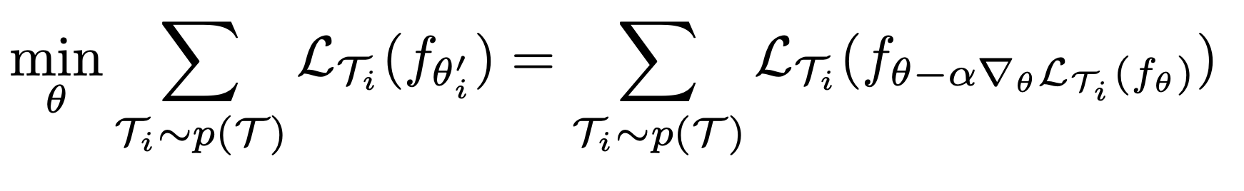
We want to find the parameters $\theta$ for our model s.t. after one step of gradient descent on new problems $T\sb{i}$, average loss is minimized.
How does MAML achieve this objective? Let’s take a look at the core algorithm. It is surprisingly simple.
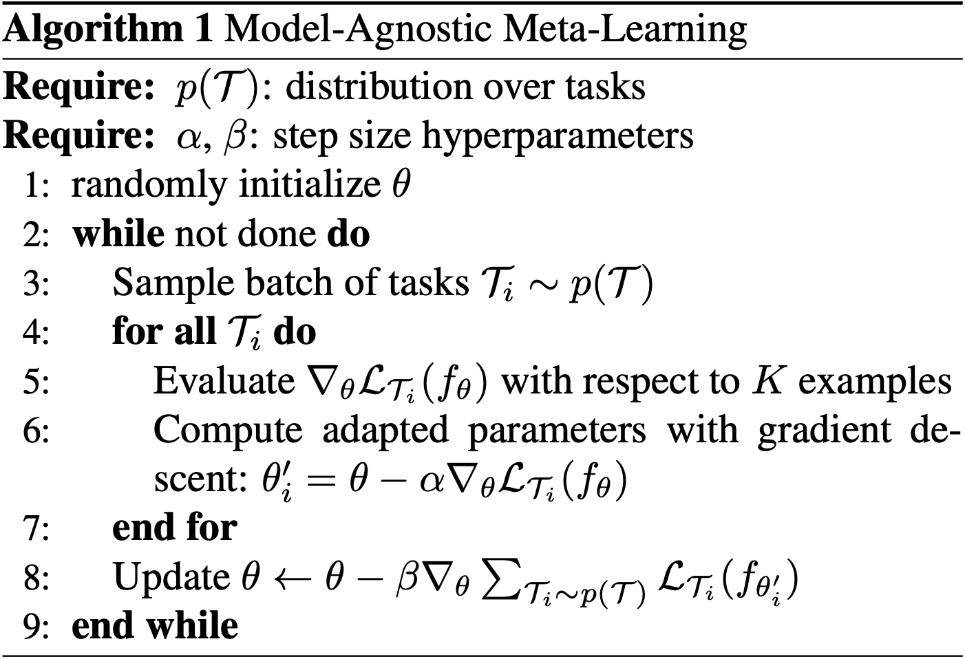
Remember, our goal is to find the best general $\theta$ for the entire distribution of tasks. We begin by sampling learning tasks from our distribution $P(T)$. For each individual task in our sample, $T\sb{i}$, we evaluate the adapted parameter $\theta^{‘}\sb{i}$. $\theta^{‘}\sb{i}$ represents the parameters of the model after performing a single step of gradient descent on a specific task $T\sb{i}$. We then perform a meta-update using gradient descent on $\theta$ to iteratively minimize the objective function.
Let’s visualize the intuition of what the algorithm is doing.
MAML has been demonstrated to produce state-of-the-art performance on certain image classification benchmarks. It also performs well on regression benchmarks and accelerates policy gradient reinforcement learning.
Applications and Use cases
Supervised Learning/Regression
MAML also can be straightforwardly extended to supervised learning.
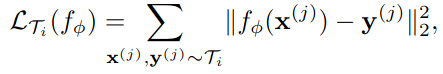
We begin by defining the horizon $H = 1$, so each data point is independent and the loss function takes a single point. Each task generates $K$ i.i.d observations $x$ from $q_i$, and loss is the error between the output for $x$ and the target values $y$.
For regression tasks using mean-squared error, the loss takes the form:
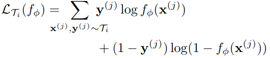
For discrete classification tasks with cross-entropy loss:
These loss functions can be inserted into Algorithm 2:
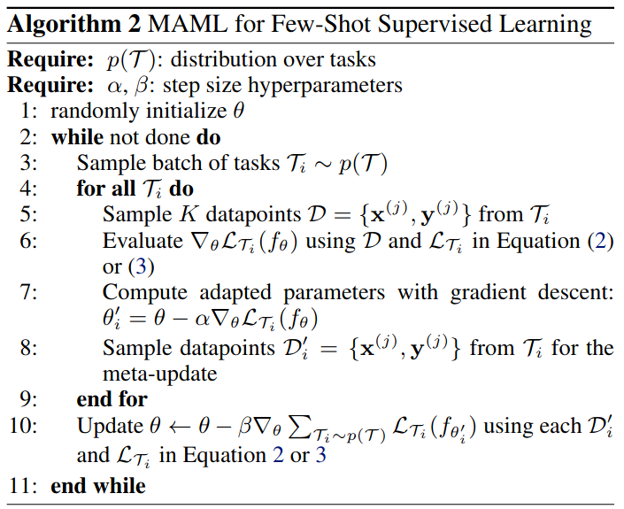
This algorithm is very similar to Algorithm 1, the general MAML algorithm. The algorithm first samples tasks from $P(T)$, the distribution on tasks. It then samples data points from each task $T\sb{i}$ to calculate the adapted parameters $\theta^{‘}\sb{i}$ for the model on each specific task. Finally, the algorithm samples more data points to iteratively change $\theta$ to minimize the average loss of the model with the adapted parameters.
Meta Reinforcement learning
In reinforcement learning, a meta-learned learner can explore more intelligently. It avoids trying useless actions and acquires the right features more quickly.
We will represent a distribution of tasks as a set of Markov Decision Processes (MDP). Each is determined a 4-tuple $\langle S, A, P_i, R_i\rangle$, where $S$ represents a set of states, $A$ represents a set of actions, $P\sb{i}: S \times A \times S \rightarrow \mathbb{R}^+$ denotes the transition probability function, and $R\sb{i}: S \times A \rightarrow \mathbb{R}$ denotes the reward function. Note that a stochastic policy $\pi\sb{\theta}: S \times A \rightarrow \mathbb{R}$ gets inputs compatible across different tasks, since a common state $S$ and action space $A$ are used. A schematic of meta-reinforcement learning that illustrates the inner and outer loops of training from Botvinick, et al. 2019 is included below. The outer loop trains the parameter weights u,which determine the inner-loop learner (’Agent’,instantiated by a recurrent neural network) that interacts with an environment for the duration of the episode. For every cycle of the outer loop, a new environment is sampled from a distribution of environments, which share some common structure.
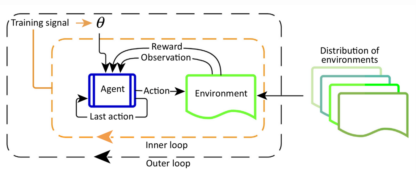
The difference between meta-RL and RL is that the last reward $r\sb{t-1}$ and the last action $a\sb{t-1}$ are incorporated into the policy observation $\pi\sb{\theta}$ in addition to the current state $s\sb{t}$. This is designed to feed history into the model so that the policy can adjust its strategy according to the states, rewards, and actions in the current MDP. The training procedure is broadly:
- Sample a new MDP from M
- Reset the hidden states of the model
- Collect trajectories and updates the model weights
- Repeat from step 1
Types of Meta-Learning Algorithms
- Optimizing Model Weights for Meta-learning: MAML and Reptile methods pre-train model parameters in order to improve performance on new tasks.
- Meta-learning Hyperparameters: Meta-gradient RL adapts to the nature of the return, or the approximation to the true value function, online while interacting and learning from the environment.
- Meta-learning the Loss Function: Evolved Policy Gradient (EPG) evolves a differentiable loss function so that the agent will achieve high rewards while minimizing the loss. The loss is parametrized via temporal convolutions over the agent’s experience. Due to the loss’s high flexibility in considering the agent’s history, fast task learning can be achieved.
- Meta-learning the exploration strategies: In model agnostic exploration with structured noise (MAESN), prior experience is used to initialize a policy and to acquire a latent exploration space that can inject structured stochasticity into a policy, which produces exploration strategies that take into account prior knowledge and are more effective than random action-space noise.
Robotics Application of Meta-RL
Meta-reinforcement learning can be used in the field of robotics. In a recent paper at the 2019 Conference on Robotic Learning, a team from Stanford, Berkley, Columbia, USC, and Google presented a paper showing their findings using meta reinforcement learning to train a Simulated Sawyer arm. They aim to meta-learn a policy that can quickly adapt to new manipulation tasks. To accomplish this, they use a few novel approaches with the following important features:
- They use the same simulated robot in all tasks.
- The observation space is always represented in the same coordinates.
- The same reward function is applied to all tasks.
- Parametric variation in object and goal positions are introduced to create an infinite variety of tasks.
The first and third requirements are in place to guarantee that tasks are within reach of single task reinforcement learning algorithms. This structure allows meta-reinforcement learning to focus on learning how to move rather than learning correspondences between the task and the robot type/reward function.
The second requirement keeps the coordinates in the observation space constant, allowing meta-learning to focus on how to move the robot without being confused by the coordinates of the space. As a whole, these first three requirements force the meta-training tasks and meta-testing tasks to be drawn from a distribution that exhibits shared structure among all tasks.
The fourth requirement differs somewhat from the first three. Parametric variation is added to induce more overlap between the tasks to prevent the algorithm from only memorizing the individual tasks. Effectively, it forces the model to learn the shared structure among the tasks, preventing overfitting and improving test performance.
Discussion and Further Work
Few-Shot Learning - Other Approaches
Few-shot learning has become popular in recent years. It aims to learn with fewer data points than standard ML algorithms. Meta-learning is one example of a few shot learning process. However, meta-learning is fairly complex. Simpler methods also produce great results. In a paper by Snell, Swersky, Zemel, “Prototypical Networks for Few-shot Learning”, they explore prototypical networks for few shot learning. The networks they describe compute representations of each class. This is done through embedding data points into a Euclidean space, based on the idea that classes of data points cluster when confined to an embedding space with fewer dimensions. Through this method, the networks are able to form boundaries for classification by looking at the data clusters. Although meta-learning has had success with few shot learning, this paper shows a new approach that not only achieves better results but also applies a simpler model. This can even be extended to zero-shot learning, which assigns each class a high level description instead of labelled data points. Zero shot learning is something that MAML may not be applicable to (yet), making prototypical networks appealing.
MAML optimization discussion
MAML aims to achieve few shot learning by only requiring a small number of gradient steps. This is a great result, but the optimization of the model parameters can be complicated. The training of the model parameters using a meta-gradient involves learning through the gradient of a gradient. This is computationally expensive, requiring the computation of a Hessian matrix at each step through additional backward passes. In recent years, methods that require a meta-gradient have become a new research focus. Many libraries like Tensorflow now support calculations like the Hessian Matrix, making the optimization easier to implement.
Another limitation of MAML is related to the distributions on tasks. MAML is dependent on knowing the probability distribution over the tasks and a probability distribution over data samples of each task. These are difficult to know \emph{a priori}.
A common problem with few-shot learning is that the model will rapidly improve for the first few gradient steps, but will overfit on a longer training horizon. Also, few-shot learning by nature does not use many data points, so it is more susceptible to overfitting. MAML bucks the trend and counteracts overfitting. The model in the MAML paper was optimized for one shot learning. In other words, the performance is maximized after one gradient step on a specific task. However, it was observed that even after continuing gradient steps, the test performance of the model continued to improve–it did not overfit. This demonstrates how MAML optimizes for fast adaptation but also can handle more training iterations without overfitting.
Meta-World: Directions for Further Work
In this robotics paper, the authors discuss possible further work. Their benchmark focuses on generalization to new tasks with new objectives. This makes it difficult to evaluate performance as previous benchmarks have a much more narrow scope.
The authors believe that much of the future work required is in algorithm design. Current meta-RL algorithms are not suited for the benchmark they have created. They also believe that their benchmark can be extended to improve its usefulness in a few ways.
- Have objects in positions that are not directly accessible to the robot.
- Consider image observations and sparse rewards.
- Include a breadth of compositional long-horizon tasks