Utilizing the HyperBand Algorithm for Hyperparameter Optimization
Published:
This is a blog post credit to Aiden Aceves, Ben Hoscheit, and Ben Stevens
The out-of-sample performance of any machine learning model hinges largely on the chosen set of hyperparameters. However, this choice is largely non-trivial as the task in hand amounts to optimizing a high-dimensional and non-convex function with unknown smoothness. As such, ad-hoc or default hyperparameter configurations are often chosen leading to sub-optimal end performance. Determining more efficient and effective ways of performing hyperparameter optimization, referred to as algorithmic configuration, is of utmost importance and has been a large focus of recent machine learning research, e.g. Hyperband, Sequential Model-based Algorithm Configuration (SMAC), genetic algorithms, and ParamILS. Moreover, associated advancements have three key practical implications:
- The development of complex algorithms can be made more efficient and less time-intensive with automatic hyperparameter optimization.
- Constructing model performance benchmarks can be done more rigorously by mitigating against sub-optimal parameter choices.
- Within fixed resource constraints, automatic hyperparameter optimization can often find a configuration leading to superior model performance as compared to ad-hoc tuning.
The two most common naive hyperparameter search strategies used in practice are grid search and random search. Grid search amounts to constructing a fixed set of hyperparameter combinations incrementing across ranges of parameters in a grid-like structure to evaluate a given model on. This approach requires an exponential number of function evaluations and therefore becomes intractable in high dimensions. Random search amounts to randomly sampling the parameter configuration space and performing model evaluation on these random configurations to determine the best configuration. However, a more rigorous class of hyperparameter optimization algorithms leveraging Bayesian optimization were thereby conceived to more intelligently probe the configuration space and attempt to scale linearly in the number of function evaluations, such as SMAC. Bayesian optimization approaches focus on configuration selection by adaptively selecting configurations to try, for example, based on constructing explicit models to describe the dependence of target algorithm performance on parameter settings such as in SMAC.
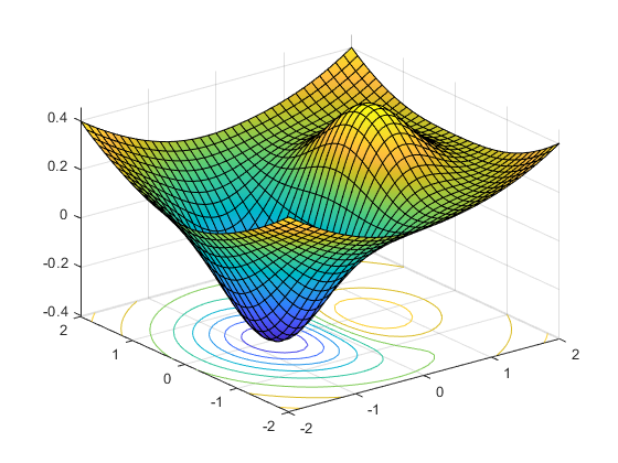
Upon further inspection, Li et al. (2018) found that when tested on a random sample of 12 benchmark algorithmic configuration datasets, approaches involving Bayesian optimization only marginally outperformed random sampling. This then led them to consider the problem of algorithmic configuration as a configuration evaluation problem thereby introducing the Hyperband algorithm. The basic idea behind the Hyperband algorithm is to utilize an adaptive resource allocation strategy based on early-stopping in order to more efficiently evaluate and explore a much larger set of random configurations compared to black-box Bayesian optimization methods: the procedure can be seen in Figure 1.
In this blog post, we aim to present the technical details of the Hyperband algorithm in a tangible way to the reader by first outlining the core algorithm and associated subroutines. We then present an example implementation of the Hyperband algorithm in an experimental setting to concretely outline a specific use-case and to reference an easy-to-use Python package available by Keras for developers.
 The numbered dots indicate successive hyperparameter configurations evaluated by the Hyperband algorithm. And the background heatmap shows the true validation error for a two-dimensional search space. The Hyperband algorithm is shown to converge to an area with the lowest validation error. (b) The Hyperband algorithm is designed to allocate more resources to promising configurations. A cutoff in resources can be seen in high loss configurations.")
Explanation of Hyperband
High-Level Description of Hyperband
Hyperband is a sophisticated algorithm for hyperparameter optimization. The creators of the method framed the problem of hyperparameter optimization as a pure-exploration, non-stochastic, infinite armed bandit problem. When using Hyperband, one selects a resource (e.g. iterations, data samples, or features) and allocates it to randomly sampled configurations. One then trains the model with each configuration, and stops training configurations that perform poorly while allocating additional resources to promising configurations.
Successive halving
Hyperband uses successive halving extensively. Successive halving works by allocating a budget to a set of hyperparameter configurations. This is done uniformly, and after this budget is depleted, half of the configurations are thrown out based on performance. The top 50% are kept and trained further with a new budget, and then 50% of these are then thrown out. The process is repeated until one configuration remains.
One downside of successive halving is that one must choose a number of configurations to input to the algorithm. So if one starts with a budget , which may be something like time or iterations, it is not always clear a priori if one should train many configurations for a short time each, or few configurations for a long time each.
More specifically, when different configurations lead to similar results, it is beneficial to use fewer configurations and train them for longer, as it will take longer to be able to accurately determine which ones are better.
Hyperband
Hyperband attempts to solve the issue with successive halving mentioned above by considering several different values for the number of configurations, , and performing a grid search over them. Each is allocated a minimum resource , with larger being assigned fewer resources (smaller ).
Hyperband has two main steps that can be viewed as a nested for loop:
The inner loop, which applies successive halving to each
The outer loop, which iterates over values of
A more detailed explanation in terms of pseudo code, taken from the Hyperband paper, can be seen below:
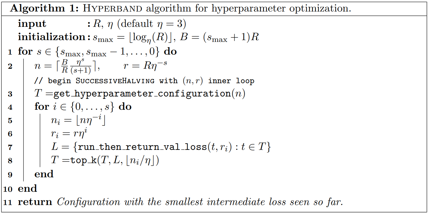
Each run of successive halving will be referred to as a bracket, and is allocated resources. So the total budget of hyperband is , where is the number of brackets.
Hyperband requires two inputs be specified: the maximum resources that can be allocated to a single configuration , and the proportion of configurations discarded each time successive halving is applied. These inputs determine how many brackets are considered. Hyperband begins with the most aggressive bracket to allow for maximum exploration. Each subsequent bracket reduces by a factor of until the final bracket when each configuration is allocated resources, which is equivalent to classical random search. This strategy allows Hyperband to exploit situations when adaptive allocations work well while maintaining adequate performance when conservative allocations are required.
Implementation
In order to implement hyperband, one must implement the following methods.
get_hyperparameter_configuration()
This function returns i.i.d. configurations from some distribution defined over the space of possible hyperparameters. One would typically use a uniform distribution, which gives a guarantee of consistency. However, if one has prior knowledge about what regions yield better hyperparameters, choosing a distribution that samples from these regions more often will improve performance.
run_then_return_val_loss(, )
This function simply takes hyperparameter configuration and resource allocation and returns the validation error.
top_k(configs, losses, )
This function simply takes a set of configurations, the losses of these configurations, and returns the best configurations.
Choosing Hyperband parameters
Choosing
As a reminder, represents the maximum amount of resources that can be allocated to any given configuration. Hence, one can typically choose this value based on what resources are available to the developer. For example, one often has an understanding of how much memory or time is available, which can help determine . One should also keep in mind that a smaller will yield faster results, while larger may yield a better configuration. If one does not have information about what should be, one can instead use the infinite horizon version of Hyperband. In the infinite horizon version, the number of unique brackets grows instead of staying constant over time.
Choosing
can be determined by practical user constraints. Larger values will cause more configurations to be eliminated each round (more aggressive), and therefore fewer rounds of eliminations. Hence, if one wants to recieve results faster they can set to be higher. The authors of the original hyperband paper note that the results are not very sensitive to , and they recommend using a value of or , although using gives the best theoretical bounds.
Theoretical Discussion of Hyperband
Hyperband has a number of nice theoretical properties. One can formalize the problem of hyperparameter optimization as a pure-exploration, non-stochastic, infinite-armed bandit (NIAB) problem. Other problems can also be formulated in this way, hence Hyperband can be applied to problems other than hyperparameter optimization.
We can formally define hyperparameter optimization as a bandit problem by considering each configuration to be an arm in the NIAB game, and consider training a configuration as a pull of that arm. Repeatedly pulling an arm yields a sequence of losses. The player can always choose to pull a new arm, or continue pulling the same arm, with no bound on the number of arms that can be drawn.
Going forward, we assume that for each configuration, the loss will converge to a fixed value if trained for an infinitely long time. We also assume that these losses are bounded and i.i.d. with CDF . We can assume that the losses are independent because the arm draws are independent, despite the fact that the validations losses do depend on the hyperparameters and most likely do correlate with certain hyperparameters. Because Hyperband does not attempt to use this information and does not assume that these correlations are structured in any specific way, the independence assumption is fine.
The object of the game is to determine which arm has the smallest fully-converged training value using the smallest number of pulls possible. Clearly, hyperparameter optimization falls under this framework. One can use this framework to derive a large number of theoretical guarantees. For example, one can prove that if sufficient resources are allocated, it will be possible to determine if one configuration is better than another. Many more theoretical results can be seen in section 5 of the Hyperband paper.
Example Implementation
We will demonstrate the hyperband algorithm using the keras-tuner package, which has implementations of several hyperparameter search algorithms. To keep the training fast, we will use MNIST, but the idea is for this to serve as a convienent entry point to adopting hyperband for your own networks.
We will start by setting up the nessecary packages. Tensorflow >= 2.0 is required. If you do not have a GPU, you can substitue the nessecary command below to use tensorflow on the CPU, but be aware that this will be slow, as we are going to train a lot of models! Also, you might want to consider installing these packages in a conda environment.
conda install tensorflow-gpu
conda install keras-tuner
We will start with a typical import of the nessecary model layers, and the Hyperband tuner.
import tensorflow as tf
from tensorflow import keras
from tensorflow.keras.datasets import mnist
from tensorflow.keras.models import Sequential
from tensorflow.keras.layers import Dense, Dropout, Flatten
from tensorflow.keras.layers import Conv2D, MaxPooling2D
from tensorflow.keras import backend as K
from tensorflow.keras.optimizers import Adam
from keras.losses import categorical_crossentropy

from kerastuner.tuners import Hyperband
The following may or may not be nessecary for your system:
gpus= tf.config.experimental.list_physical_devices('GPU')
tf.config.experimental.set_memory_growth(gpus[0], True)
First we construct a baseline network as demonstrated in the keras examples. Note that this will automatically download the mnist dataset if you do not already have it.
Partition the data training & test sets:
num_classes = 10

# the data, split between train and test sets
(x_train, y_train), (x_test, y_test) = mnist.load_data()

x_train = x_train.reshape(x_train.shape[0], 28, 28, 1)
x_test = x_test.reshape(x_test.shape[0], 28, 28, 1)
input_shape = (28, 28, 1)

x_train = x_train.astype('float32')
x_test = x_test.astype('float32')
x_train /= 255
x_test /= 255
print('x_train shape:', x_train.shape)
print(x_train.shape[0], 'train samples')
print(x_test.shape[0], 'test samples')

# convert class vectors to binary class matrices
y_train = keras.utils.to_categorical(y_train, num_classes)
y_test = keras.utils.to_categorical(y_test, num_classes)
x_train shape: (60000, 28, 28, 1)
60000 train samples
10000 test samples
Build the model, and train it:
model = Sequential()
model.add(Conv2D(32, kernel_size=(3, 3),
                 activation='relu',
                 input_shape=input_shape))
model.add(Conv2D(64, (3, 3), activation='relu'))
model.add(MaxPooling2D(pool_size=(2, 2)))
model.add(Dropout(0.3))
model.add(Flatten())
model.add(Dense(128, activation='relu'))
model.add(Dropout(0.5))
model.add(Dense(num_classes, activation='softmax'))

model.compile(loss='categorical_crossentropy',
              optimizer=Adam(),
              metrics=['accuracy'])

batch_size = 128
epochs = 12

model.fit(x_train, y_train,
          batch_size=batch_size,
          epochs=epochs,
          verbose=0,
          validation_data=(x_test, y_test))
score = model.evaluate(x_test, y_test, verbose=0)
print('Test loss:', score[0])
print('Test accuracy:', score[1])
Test loss: 0.028736516343067522
Test accuracy: 0.9917
This basic model achieves ~99.25% accuracy in 12 epochs.
Now we will try the same task using the keras-tuning module. The hyperband tuner will need to be passed a function that returns a keras model. For each of the hyperparameters that we wish to tune, we will pass a placeholder value of type “Choice”, “Float” or “Int”. Each of these placeholders will specify a name, a range of values to search, a default value, and for Floats, a step size. More hyperparameter placeholds are available too: keras-tuner documentation.
def MNISTHyperModel(hp):
    num_classes = 10
    model = keras.Sequential()

    model.add(Conv2D(
            filters=hp.Choice('num_filters_1', values=[16, 32, 64], default = 32),
            kernel_size=hp.Choice('kernel_1', values=[2,3,4,5], default = 3),
            strides = hp.Choice('stride_1', values=[1,2,3], default = 1),
            activation = 'relu',
            input_shape=(28,28,1)))

    model.add(Conv2D(
            filters=hp.Choice('num_filters_2', values=[16, 32, 64], default = 32),
            kernel_size=hp.Choice('kernel_2', values=[2,3,4,5], default = 3),
            strides = hp.Choice('stride_2', values=[1,2,3], default = 1),
            activation='relu'))

    model.add(MaxPooling2D(pool_size=2))

    model.add(Dropout(rate=hp.Float('dropout_1', min_value=0.0, max_value=0.5, default=0.3, step=0.1)))

    model.add(Flatten())

    model.add(Dense(
            units=hp.Int('dense_units', min_value=32, max_value=512, step=32, default=128),
            activation=hp.Choice('dense_activation', values=['relu', 'tanh', 'sigmoid'], default='relu')))

    model.add(Dropout(rate=hp.Float('dropout_2', min_value=0.0, max_value=0.5, default=0.5, step=0.1)))
    model.add(Dense(num_classes, activation='softmax'))

    model.compile(
        optimizer=Adam(
            hp.Float('learning_rate', min_value=1e-4, max_value=1e-2, sampling='LOG', default=1e-3)),
        loss='categorical_crossentropy',
        metrics=['accuracy'])
    return model
Note that we have specified that the learning rate should be explored equally accross each order of magnitude range.
Now we will setup the tuner object, which will run the hyperband algorithm. We set the max epochs to 12, the same as the baseline example above, but in reality this number should be larger. We also specify that we want the model with the best validation accuracy, and that all models should be evaluated in triplicate. Directory and project name will be used for a folder and subfolder (respectively) to hold the results.
tuner = Hyperband(
    MNISTHyperModel,
    max_epochs=12,
    objective='val_accuracy',
    executions_per_trial=3,
    directory='hyperband',
    project_name='MNIST_hyperband_2')
To review the search space to be searched by the model run:
tuner.search_space_summary()
Now we will kick off the training. This took about an hour on a modern GPU (Titan V)
tuner.search(x_train, y_train, validation_split=0.1)
Once that completes, we can show a summary of the search:
tuner.results_summary()
We can get the best model, and test it out on the same split as before:
best_model = tuner.get_best_models(num_models=1)[0]
loss, accuracy = best_model.evaluate(x_test, y_test)
print(accuracy)
0.9927
About the same as the basic model! Not too surprising given the relative simplicity of the problem, and the low number of epochs.
Let’s examine the model:
best_model.summary()
Model: "sequential"
_________________________________________________________________
Layer (type)                 Output Shape              Param #
=================================================================
conv2d (Conv2D)              (None, 26, 26, 16)        160
_________________________________________________________________
conv2d_1 (Conv2D)            (None, 24, 24, 16)        2320
_________________________________________________________________
max_pooling2d (MaxPooling2D) (None, 12, 12, 16)        0
_________________________________________________________________
dropout (Dropout)            (None, 12, 12, 16)        0
_________________________________________________________________
flatten (Flatten)            (None, 2304)              0
_________________________________________________________________
dense (Dense)                (None, 384)               885120
_________________________________________________________________
dropout_1 (Dropout)          (None, 384)               0
_________________________________________________________________
dense_1 (Dense)              (None, 10)                3850
=================================================================
Total params: 891,450
Trainable params: 891,450
Non-trainable params: 0
_________________________________________________________________
Much more detailed results can be found in the output folders of the specific runs (we named this folder earlier), including the preformance in each round, and what models “made the cut” in each round.
Final Thoughts
In this blog post, we introduced the problem of hyperparameter optimization within the context of machine learning. We discussed the practical importance of solutions in the development of complex algorithms, constructing model performance benchmarks, and finding the best hyperparamter configuration in a fixed resource context. We then outlined some well-known and well-practiced solutions in random search, grid search, those involving Bayesian optimization, and then th HyperBand algorithm. We focused on describing the technical components of the HyperBand algorithm, and its associated subroutines and theory. Finally, we presented an example implementation of the Hyperband algorithm in an experimental setting to concretely outline a specific use-case and to reference an easy-to-use Python package available by Keras for developers.