Learning to optimize in learning

This is a blog post credit to Alvin On and Mario Ruiz

Optimization is a core component of Machine Learning. Nearly every machine learning task can be framed as an optimization problem. Given some objective function or loss function that is used to evaluate a model’s performance on the task at hand, we can recontextualize the machine learning task as an optimization problem—we are searching for the set of model parameters that minimizes the value of this objective function.

Over the years, a great deal of effort has been put towards discovering new and better optimizers for model training. The most classic of techniques, Stochastic Gradient Descent (SGD), uses the gradient of the objective function to update model parameters. Momentum improves upon SGD by looking at a series of previously computed gradients to get a better idea of the overall shape of the optimization surface in order to move faster towards convergence. Adagrad adjusts the learning rate individually for each parameter so that infrequent parameters are updated in larger steps while frequent parameters are updated in smaller steps. RMSProp is an improvement over Adagrad that adjusts the learning rate for each parameter without rapidly diminishing the overall learning rate. Finally, Adam is a combination of Adagrad and RMSProp that uses estimates of the first and second moment of gradients to calculate learning rates for each parameter.

Learning an Optimizer

Designing optimization algorithms is a difficult and tedious process. Additionally, most optimization algorithms are designed to generalize to a variety of different machine learning problems and architectures. This limits their ability to exploit more problem specific structure and information to further improve performance.

However, what if we could learn the optimization process? Rather than hand crafting generalized update rules, we could instead train a model to learn its own update rules. We could train this optimizer on specific types of machine learning problems, allowing it to learn more effective update rules that are better able to exploit problem specific information, all while avoiding having to design our own update rules.

First we’ll examine some popular optimizers used today to get a better idea of what an update rule looks like. Taking a closer look at the Adam and RMSProp optimizers, we can see the importance of storing additional information across different optimization steps. This additional information is used to supplement the gradient and provide a better update step calculation. For example, stores first and second moment vectors while RMSProp stores an average of the squares of previously computed gradients. Both algorithms use this additional information to adjust the step size of the different model parameters. With this in mind, we can generalize the update step to something like the following:

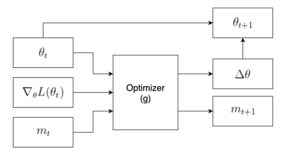
In the figure above, $\theta_t$ represents the current “state” of the optimization problem, which could be the current values of the model parameters we are attempting to learn. The $\nabla_{\theta} L(\theta_t)$ is the gradient of the loss function with respect to the current state. The last parameter. $m_t$, represents the “memory” of our optimizer. Any persistent values we need to keep across different iteration, such as a cumulative sum of previously computed gradients, can be stored in this variable. Finally, the function $g$ represents our optimization algorithm.

Our end goal is to replace $g$ with some machine learning model that is able to learn an optimal optimization algorithm. Examining the structure of the update step, we can see that it resembles a recurrent neural network (RNN).

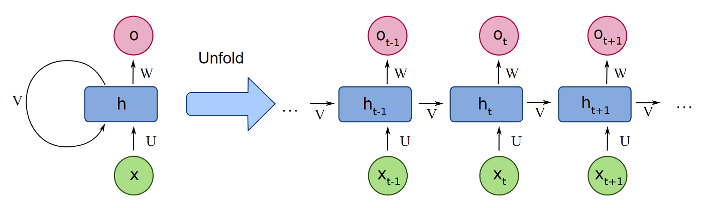
An RNN is a special type of neural network that updates a hidden internal state based on the output of the previous input. It is useful for problems where we need to calculate the outputs for a sequence of inputs, and we need to keep track of information from previous inputs. In the case of our optimizer, given a series of problem states, $\theta_t$, we want to compute a series of update steps while keeping track of some sort of internal memory.

Training the optimizer

In order to train this optimizer RNN, we need some sort of loss function to evaluate the optimizer’s performance. Let $\phi$ be the parameters for our optimizer and $\theta^{*}(f, \phi)$ be the final optimized parameters the optimizer returns for an objective function $f$. Naively, an optimizer’s performance should be evaluated by these final parameters, giving us the loss function

However, training with this loss function is difficult, since we only have information from the very last output of the optimizer and no information from the path we took to get to this final value. Incorporating information from each step of the optimization would allow for more efficient training, giving us the modified loss function

where $\theta_t$ is the parameters returned by the optimizer at update $t$ and $T$ is the total number of updates.

Another problem with RNNs arises as we increase the size of the model we are learning to optimize. At the scale of tens of thousands of parameters, training a fully connected RNN becomes infeasible due to the enormous amount of parameters it would require. To combat this problem, we make our optimizer operate coordinatewise on the parameters of the model we are optimizing. This way, we can share RNN parameters across different parameters of the model we are optimizing, resulting in a greatly reduced parameter count.

Results

In their paper, “Learning to learn by gradient descent by gradient descent”, Andrychowicz et al introduce the method described above to train an optimizer. The authors used two layer LSTMs with 20 hidden units in each layer, using ADAM to minimize the objective function described above.

The authors first trained the LSTM optimizer on a single layer, 20 hidden unit feedforward network learning the MNIST dataset. They compared the LSTM optimizer’s performance against several other popular optimizers. The results are show below.

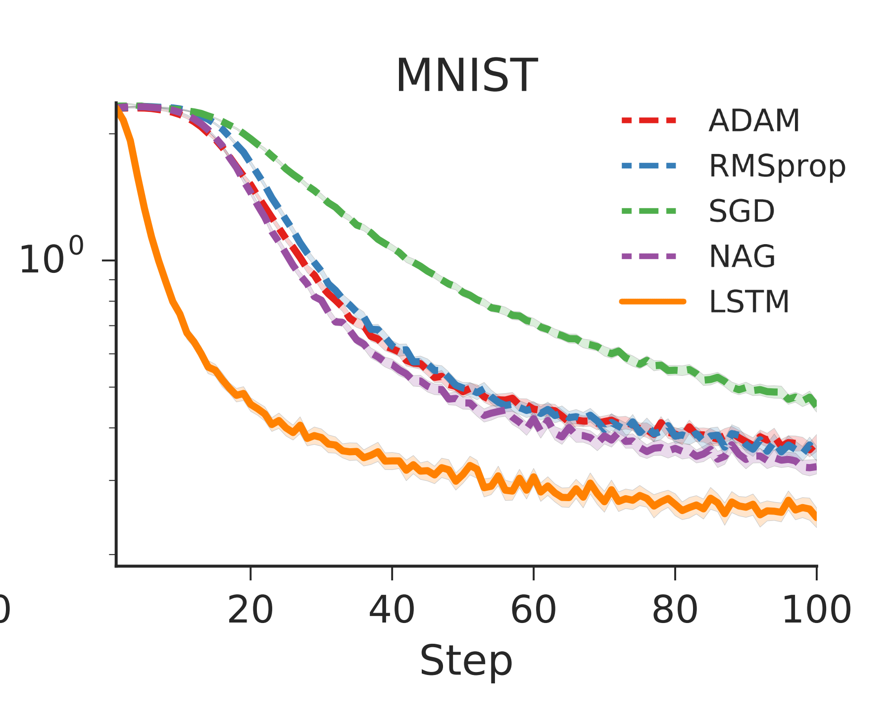
The results look promising for this first test, with the LSTM outperforming the other optimizers.

The authors then tested how well the LSTM optimizer generalized to neural networks with different architectures. They tried varying the number of hidden layers, the number of units, and even the activation function of the network. The results are show below.

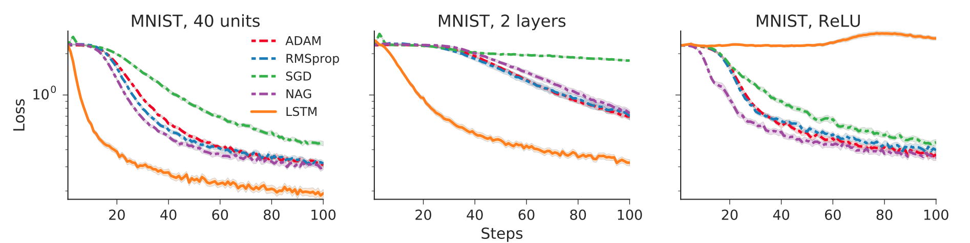
As we can see, the LSTM optimizer generalized well when varying the number of units and layers, but did not generalize to a new activation.

OptNet

Beyond training a machine learning model, machine learned optimizers can also be applied to general optimization tasks that fit the same parameters. For the generalized SGD with momentum optimizer described earlier, we can theoretically apply it to any interface that computes a gradient to minimize; so more than just machine learning models. In addition, these learned optimizers can be taught to solve different kinds of optimization problems. Given these new perspectives, we can treat differentiable optimization as a modular tool; and not only use these learned optimizers on our deep learning models, but also in conjunction with our deep learning model to optimize other tasks. In this section, we will step away from learned optimizers and instead look at OptNet, which learns an instance of a quadratic programming problem to better approximate possible constraints for a given task.

What is OptNet?

OptNet is introduced by Amos and Kolter in their paper: “OptNet: Differentiable Optimization as a Layer in Neural Networks”. The paper describes OptNet as:

“A network architecture that integrates optimization problems (here, specifically in the form of quadratic programs) as individual layers in larger end-to-end trainable deep networks.”

Essentially, OptNet integrates an optimization problem directly into your deep learning model. As stated in the quote above, although they specifically use quadratic programming in the theoretical and empirical analysis of their paper, OptNet can be applied to general optimization problems.

The basic structure of the OptNet layer is to treat the optimization parameters as learnable functions in terms of the layer input. The layer output is then the solution to the resulting optimization problem. This relationship is modeled by the given quadratic problem:

Before examining the equation, let’s rewrite it using a slightly more suggestive notation (which is also easier to type!).

In this form, we treat $x = z_i$ as the output of the previous layer. This term is given to us as an input of this layer, and we can use it later to compute backwards and forward gradients for training the optimization constraints. We shorten $z = z_{i+1}$ as the output of this OptNet layer, which is the solution to the quadratic problem above. Thus, our explanation of the layer architecture is complete!

Training an OptNet Layer

The authors of the paper describe an intelligent way to learn the optimization constraints and solve the optimizations efficiently on parallel hardware. However, that is not the main focus of this post, so we will only briefly gloss over these topics. The paper itself is (obviously) an amazing resource for analyzing these points in greater depth. For learning the optimization constraints, the authors make use of the KKT conditions for quadratic problems to solve for differentials of the output term, $d z$, and the primal and dual factors $d \lambda$ and $d \nu$. Once these differentials are given, we can determine the total gradient over each of the optimization constraints in terms of the differentials. The authors introduce a shortcut for computing the gradient in the backwards pass by using the KKT conditions at the existing solution that was already solved during the forward pass.

Using OptNet: Sudoku Solver

This OptNet layer has one major strength that makes it very proficient at solving certain types of deep learning tasks: it is able to learn complex patterns in large search space that helps during training to narrow down onto better solutions. A prime example of a complex problem of this nature is solving a sudoku board. If told the rules of the game, sudoku becomes trivial for computers to solve as a constraint satisfaction problem. However, if only given starting and solved boards, we are given a very non-obvious transformation that our model is trying to replicate.

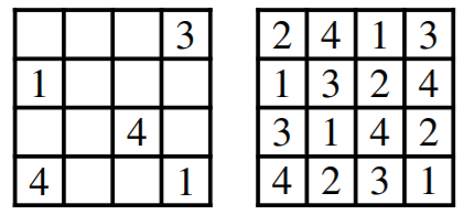
Figure 1: Example of a sudoku board and it’s solution (from Amos and Kolter)

We can actually make this transformation easier to find by taking advantage of one simple fact: we know that the game has constraints. Normally, a programmer would manually determine these constraints then conjure up a solution that works around it. However, OptNet allows us to learn the constraints as an integral part of the model itself. By learning the proper constraints for the sudoku problem, it becomes easier for the model to solve it; as it can simply pass a feature representation of the board to the optimization layer, and then using the optimal solution of that layer to solve the overall problem.

The results of this experiment (conducted by Amos and Kolter) are shown in the graphs below. As we can see, a standard convolutional network overfits on the sudoku problem (test error is much higher than training error). This is because there are many possible mappings that could transform a given starting board to a solution board based on computation alone. Thus, there is a large space of plausible solutions (within an error range) for a given training set, which don’t necessarily imply a solution for the test set. These would be mappings that can’t understand the constraints of the sudoku problem, and instead just find some way to “convert these numbers to the others”. On the other hand, the OptNet model seems to begin learning the sudoku problem much earlier in training, and does not overfit (the test and training errors are approximately the same). As mentioned earlier, this is because it directly considers constraints as a part of it’s architecture.

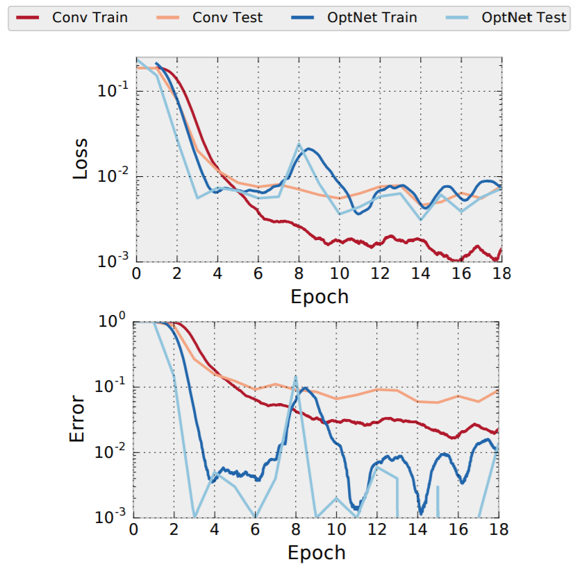
Figure 2: Training and Test errors for a convolutional model vs. OptNet (from Amos and Kolter)

Combining OptNet with a Learned Optimizer

Sudoku is known to be solvable using integer programming, but what about other tasks that have different optimizers or constraints? As mentioned above OptNet can be used for general optimization methods, but it is not guaranteed that these methods are easy to compute efficiently. It may be the case that the constraint class for a problem becomes very hard and inefficient to compute.

Thus, we return back to learned optimizers. In place of manually performing the optimization search, we can use a learned optimizer to directly compute a (near) optimal value for the OptNet layer. If our learned optimizer can give us a near-optimal result while computing an overall faster computation in total, then we can improve the total evaluation speed of our model. A combined approach like this may be able to improve the evaluation speed of a model, while also allowing it to solve very high dimensional problems without increasing our model size too much.